读取 MAPDL 结果文件

Reading MAPDL Result Files

ansys-mapdl-reader 模块支持 MAPDL 的以下结果类型：

• ".rfl"

• ".rmg"

• ".rst" - Structural analysis result file 结构分析结果文件

• ".rth"

MAPDL 结果文件是 FORTRAN 格式的二进制文件，包含从 MAPDL 分析写入的结果。结果至少包含分析模型的几何结构以及节点和单元结果。 根据分析，这些结果可以是从模态位移到节点温度的任何结果。这包括（但不限于）：

• 节点自由度结果，来自静态分析或模态分析。

• 节点自由度结果，来自循环静态或模态分析。

• 节点平均分量应力（即 x、y、z、xy、xz、yz）

• 节点主应力（即 S1、S2、S3、SEQV、SINT）

• 节点弹性、塑性和热应力

• 节点时程结果

• 节点边界条件和力

• 节点温度

• 节点热应变

• 各种单元结果（请参见 element_solution_data ）

该模块将来可能会被弃用，我们建议您查看 DPF-Core 和 DPF-Post 的新数据处理框架（DPF）模块， 因为它们使用客户端/服务器端接口，使用与 ANSYS Workbench 中相同的软件，但通过 Python 客户端，为 ANSYS 结果文件提供了一个更现代化的接口。

加载结果文件

由于 MAPDL 结果文件是二进制文件，因此无需将整个文件加载到内存中就能获取结果。该模块通过一个 python 对象 result 访问结果，您可以使用该对象 result 进行初始化：

from ansys.mapdl import reader as pymapdl_reader
result = pymapdl_reader.read_binary('file.rst')

初始化时， Result 对象包含几个属性，其中包括分析的时间值、节点编号、单元编号等。

ansys-mapdl-reader 模块可以通过读取 ‘the header of the file’ 来确定正确的结果类型， 这意味着如果是 MAPDL 二进制文件， ansys-mapdl-reader 可能可以读取（至少在某种程度上）。 例如，可以使用以下命令读取热分析结果文件

rth = pymapdl_reader.read_binary('file.rth')

结果属性

通过打印结果文件，可以快速显示 Result 的属性：

>>> result = pymapdl_reader.read_binary('file.rst')
>>> print(result)
PyMAPDL Result file object
Units       : User Defined
Version     : 20.1
Cyclic      : False
Result Sets : 1
Nodes       : 321
Elements    : 40


Available Results:
EMS : Miscellaneous summable items (normally includes face pressures)
ENF : Nodal forces
ENS : Nodal stresses
ENG : Element energies and volume
EEL : Nodal elastic strains
ETH : Nodal thermal strains (includes swelling strains)
EUL : Element euler angles
EPT : Nodal temperatures
NSL : Nodal displacements
RF  : Nodal reaction forces

要获取分析的时间或频率值，请使用

>>> result.time_values
array([1.])

可以使用 result 对象的多种可用方法之一获取单个结果。例如，第一个结果的节点位移可以这样用：

>>> nnum, disp = rst.nodal_displacement(0)
>>> nnum
array([  1,   2,   3, ..., 318, 319, 320, 321], dtype=int32)

>>> disp
array([[-2.03146520e-09, -3.92491045e-03,  5.00047448e-05],
       [ 1.44630651e-09,  1.17747356e-02, -1.49992672e-04],
       [ 0.00000000e+00,  0.00000000e+00,  0.00000000e+00],
       ...
       [-7.14982194e-03,  3.12495002e-03,  5.74992265e-04],
       [-7.04982329e-03,  2.44996706e-03,  5.74992939e-04],
       [-6.94982520e-03,  1.77498362e-03,  5.74992891e-04]])

可以通过以下方法获得结果的节点排序和单元编号：

>>> rst.geometry.nnum
array([  1,   2,   3, ..., 318, 319, 320, 321], dtype=int32)

>>> result.geometry.enum
array([ 1,  3,  2,  4,  5,  7,  6,  8,  9, 11, 10, 12, 13, 15, 14, 16, 17,
       19, 18, 20, 21, 23, 22, 24, 25, 27, 26, 28, 29, 31, 30, 32, 33, 35,
       34, 36, 37, 39, 38, 40], dtype=int32)

Mesh

查询结果的 mesh 属性可找到结果的网格，该属性会返回一个 ansys.mapdl.reader.mesh.Mesh 类。

>>> from ansys.mapdl import reader as pymapdl_reader
>>> from ansys.mapdl.reader import examples
>>> rst = pymapdl_reader.read_binary(examples.rstfile)
>>> print(rst.mesh)

ANSYS Mesh
  Number of Nodes:              321
  Number of Elements:           40
  Number of Element Types:      1
  Number of Node Components:    0
  Number of Element Components: 0

其中包含以下属性：

class ansys.mapdl.reader.mesh.Mesh(nnum=None, nodes=None, elem=None, elem_off=None, ekey=None, node_comps={}, elem_comps={}, rdat=[], rnum=[], keyopt={})

Common class between Archive, and result mesh

property ekey

Element type key

Array containing element type numbers in the first column and the element types (like SURF154) in the second column.

Examples

>>> from ansys.mapdl import reader as pymapdl_reader
>>> from ansys.mapdl.reader import examples
>>> archive = pymapdl_reader.Archive(examples.hexarchivefile)
>>> archive.ekey
array([[  1,  45],
       [  2,  95],
       [  3,  92],
       [ 60, 154]], dtype=int32)

property elem

List of elements containing raw ansys information.

Each element contains 10 items plus the nodes belonging to the element. The first 10 items are:

• FIELD 0 : material reference number

• FIELD 1 : element type number

• FIELD 2 : real constant reference number

• FIELD 3 : section number

• FIELD 4 : element coordinate system

• FIELD 5 : death flag (0 - alive, 1 - dead)

• FIELD 6 : solid model reference

• FIELD 7 : coded shape key

• FIELD 8 : element number

• FIELD 9 : base element number (applicable to reinforcing elements only)

• FIELDS 10 - 30 : The nodes belonging to the element in ANSYS numbering.

Examples

>>> from ansys.mapdl import reader as pymapdl_reader
>>> from ansys.mapdl.reader import examples
>>> archive = pymapdl_reader.Archive(examples.hexarchivefile)
>>> archive.elem
[array([  1,   4,  19,  15,  63,  91, 286, 240,   3,  18,  17,
         16,  81, 276, 267, 258,  62,  90, 285, 239],
 array([  4,   2,   8,  19,  91,  44, 147, 286,   5,   7,  21,
         18, 109, 137, 313, 276,  90,  43, 146, 285],
 array([ 15,  19,  12,  10, 240, 286, 203, 175,  17,  20,  13,
         14, 267, 304, 221, 230, 239, 285, 202, 174],
...

property elem_real_constant

Real constant reference for each element.

Use the data within rlblock and rlblock_num to get the real constant datat for each element.

Examples

>>> from ansys.mapdl import reader as pymapdl_reader
>>> from ansys.mapdl.reader import examples
>>> archive = pymapdl_reader.Archive(examples.hexarchivefile)
>>> archive.elem_real_constant
array([ 1,  1,  1,  1,  1,  1,  1,  1,  1,  1,  1,  1,  1,  1,
        1,  1,  1,  1,  1,  1,  1,  1,  1,  1,  1,  1,  1,  1,
        1,  1,  1,  1,  1,  1,  1,  1,  1,  1,  1,  1,  1,  1,
        ...,
        1,  1,  1,  1,  1,  1,  1,  1,  1,  1, 61, 61, 61, 61,
       61, 61, 61, 61, 61, 61, 61, 61, 61, 61, 61, 61, 61, 61,
       61], dtype=int32)

property element_components

Element components for the archive.

Output is a dictionary of element components. Each entry is an array of MAPDL element numbers corresponding to the element component. The keys are element component names.

Examples

>>> from ansys.mapdl import reader as pymapdl_reader
>>> from ansys.mapdl.reader import examples
>>> archive = pymapdl_reader.Archive(examples.hexarchivefile)
>>> archive.element_components
{'ECOMP1 ': array([17, 18, 21, 22, 23, 24, 25, 26, 27, 28, 29,
                   30, 31, 32, 33, 34, 35, 36, 37, 38, 39, 40],
                   dtype=int32),
'ECOMP2 ': array([ 1, 2, 3, 4, 5, 6, 7, 8, 9, 10, 11, 12, 13,
                  14, 15, 16, 17, 18, 19, 20, 23, 24], dtype=int32)}

element_coord_system()

Element coordinate system number

Examples

>>> from ansys.mapdl import reader as pymapdl_reader
>>> from ansys.mapdl.reader import examples
>>> archive = pymapdl_reader.Archive(examples.hexarchivefile)
>>> archive.element_coord_system
array([0, 0, 0, 0, 0, 0, 0, 0, 0, 0, 0, 0, 0, 0, 0, 0, 0, 0, 0,
       0, 0, 0, 0, 0, 0, 0, 0, 0, 0, 0, 0, 0, 0, 0, 0, 0, 0, 0,
       0, 0], dtype=int32)

property enum

ANSYS element numbers.

Examples

>>> from ansys.mapdl import reader as pymapdl_reader
>>> from ansys.mapdl.reader import examples
>>> archive = pymapdl_reader.Archive(examples.hexarchivefile)
>>> archive.enum
array([    1,     2,     3, ...,  9998,  9999, 10000])

property et_id

Element type id (ET) for each element.

property etype

Element type of each element.

This is the ansys element type for each element.

Examples

>>> from ansys.mapdl import reader as pymapdl_reader
>>> from ansys.mapdl.reader import examples
>>> archive = pymapdl_reader.Archive(examples.hexarchivefile)
>>> archive.etype
array([ 45,  45,  45,  45,  45,  45,  45,  45,  45,  45,  45,
        45,  45,  45,  45,  45,  45,  45,  45,  92,  92,  92,
        92,  92,  92,  92,  92,  92,  92,  92,  92,  92,  92,
        ...,
        92,  92,  92,  92,  92, 154, 154, 154, 154, 154, 154,
       154, 154, 154, 154, 154, 154, 154, 154, 154, 154, 154,
       154], dtype=int32)

Notes

Element types are listed below. Please see the APDL Element Reference for more details:

https://www.mm.bme.hu/~gyebro/files/vem/ansys_14_element_reference.pdf

property key_option

Additional key options for element types

Examples

>>> from ansys.mapdl import reader as pymapdl_reader
>>> from ansys.mapdl.reader import examples
>>> archive = pymapdl_reader.Archive(examples.hexarchivefile)
>>> archive.key_option
{1: [[1, 11]]}

property material_type

Material type index of each element in the archive.

Examples

>>> from ansys.mapdl import reader as pymapdl_reader
>>> from ansys.mapdl.reader import examples
>>> archive = pymapdl_reader.Archive(examples.hexarchivefile)
>>> archive.material_type
array([1, 1, 1, 1, 1, 1, 1, 1, 1, 1, 1, 1, 1, 1, 1, 1, 1, 1,
       1, 1, 1, 1, 1, 1, 1, 1, 1, 1, 1, 1, 1, 1, 1, 1, 1, 1,
       1, 1, 1, 1], dtype=int32)

property n_elem

Number of nodes

property n_node

Number of nodes

property nnum

Array of node numbers.

Examples

>>> from ansys.mapdl import reader as pymapdl_reader
>>> from ansys.mapdl.reader import examples
>>> archive = pymapdl_reader.Archive(examples.hexarchivefile)
>>> archive.nnum
array([    1,     2,     3, ..., 19998, 19999, 20000])

property node_angles

Node angles from the archive file.

Examples

>>> from ansys.mapdl import reader as pymapdl_reader
>>> from ansys.mapdl.reader import examples
>>> archive = pymapdl_reader.Archive(examples.hexarchivefile)
>>> archive.nodes
[[0.   0.   0.  ]
 [0.   0.   0.  ]
 [0.   0.   0.  ]
 ...,
 [0.   0.   0.  ]
 [0.   0.   0.  ]
 [0.   0.   0.  ]]

property node_components

Node components for the archive.

Output is a dictionary of node components. Each entry is an array of MAPDL node numbers corresponding to the node component. The keys are node component names.

Examples

>>> from ansys.mapdl import reader as pymapdl_reader
>>> from ansys.mapdl.reader import examples
>>> archive = pymapdl_reader.Archive(examples.hexarchivefile)
>>> archive.node_components
{'NCOMP2  ': array([  1,   2,   3,   4,   5,   6,   7,   8,
                     14, 15, 16, 17, 18, 19, 20, 21, 43, 44,
                     62, 63, 64, 81, 82, 90, 91, 92, 93, 94,
                     118, 119, 120, 121, 122, 123, 124, 125,
                     126, 137, 147, 148, 149, 150, 151, 152,
                     153, 165, 166, 167, 193, 194, 195, 202,
                     203, 204, 205, 206, 207, 221, 240, 258,
                     267, 268, 276, 277, 278, 285, 286, 287,
                     304, 305, 306, 313, 314, 315, 316
                     ], dtype=int32),
...,
}

property nodes

Array of nodes.

Examples

>>> from ansys.mapdl import reader as pymapdl_reader
>>> from ansys.mapdl.reader import examples
>>> archive = pymapdl_reader.Archive(examples.hexarchivefile)
>>> archive.nodes
[[0.   0.   0.  ]
 [1.   0.   0.  ]
 [0.25 0.   0.  ]
 ...,
 [0.75 0.5  3.5 ]
 [0.75 0.5  4.  ]
 [0.75 0.5  4.5 ]]

property rlblock

Real constant data from the RLBLOCK.

Examples

>>> from ansys.mapdl import reader as pymapdl_reader
>>> from ansys.mapdl.reader import examples
>>> archive = pymapdl_reader.Archive(examples.hexarchivefile)
>>> archive.rlblock
[[0.   , 0.   , 0.   , 0.   , 0.   , 0.   , 0.02 ],
 [0.   , 0.   , 0.   , 0.   , 0.   , 0.   , 0.01 ],
 [0.   , 0.   , 0.   , 0.   , 0.   , 0.   , 0.005],
 [0.   , 0.   , 0.   , 0.   , 0.   , 0.   , 0.005]]

property rlblock_num

Indices from the real constant data

Examples

>>> from ansys.mapdl import reader as pymapdl_reader
>>> from ansys.mapdl.reader import examples
>>> archive = pymapdl_reader.Archive(examples.hexarchivefile)
>>> archive.rnum
array([60, 61, 62, 63])

save(filename, binary=True, force_linear=False, allowable_types=[], null_unallowed=False)

Save the geometry as a vtk file

Parameters:

• filename (str, pathlib.Path) – Filename of output file. Writer type is inferred from the extension of the filename.

• binary (bool, optional) – If True, write as binary, else ASCII.

• force_linear (bool, optional) – This parser creates quadratic elements if available. Set this to True to always create linear elements. Defaults to False.

• allowable_types (list, optional) –

  Allowable element types. Defaults to all valid element types in ansys.mapdl.reader.elements.valid_types

  See help(ansys.mapdl.reader.elements) for available element types.

• null_unallowed (bool, optional) – Elements types not matching element types will be stored as empty (null) elements. Useful for debug or tracking element numbers. Default False.

Examples

>>> geom.save('mesh.vtk')

Notes

Binary files write much faster than ASCII and have a smaller file size.

property section

Section number

Examples

>>> from ansys.mapdl import reader as pymapdl_reader
>>> from ansys.mapdl.reader import examples
>>> archive = pymapdl_reader.Archive(examples.hexarchivefile)
>>> archive.section
array([1, 1, 1, 1, 1, 1, 1, 1, 1, 1, 1, 1, 1, 1, 1, 1, 1, 1, 1,
       1, 1, 1, 1, 1, 1, 1, 1, 1, 1, 1, 1, 1, 1, 1, 1, 1, 1, 1,
       1, 1], dtype=int32)

property tshape

Tshape of contact elements.

property tshape_key

Dict with the mapping between element type and element shape.

TShape is only applicable to contact elements.

坐标系

非默认坐标系始终保存到 MAPDL 结果文件中。坐标系为零索引，可以通过以下方式访问各个坐标系：

>>> coord_idx = 12
>>> result.geometry['coord systems'][coord_idx]
{'transformation matrix': array([[ 0.0, -1.0,  0.0],
                                 [ 0.0,  0.0, -1.0],
                                 [ 1.0,  0.0,  0.0]]),
 'origin': array([0., 0., 0.]),
 'PAR1': 1.0,
 'PAR2': 1.0,
 'euler angles': array([ -0., -90.,  90.]),
 'theta singularity': 0.0,
 'phi singularity': 0.0,
 'type': 1,
 'reference num': 12}

可以通过将变换矩阵和原点连接成一个数组来构造 4x4 变换矩阵。例如：

>>> cs = result.geometry['coord systems'][coord_idx]
>>> trans = cs['transformation matrix']
>>> origin = cs['origin']
>>> bottom = np.zeros(4)
>>> bottom[3] = 1
>>> tmat = np.hstack((trans, origin.reshape(-1 ,1)))
>>> tmat = np.vstack((tmat, bottom))

有关结果文件中存储的坐标系内容的更多详情，请参阅 parse_coordinate_system 。

访问求解结果

您可以使用 solution_info 获取每个 result 的详细信息：

# 返回第一个 result 的 solution 信息字典
info = result.solution_info(0)

for key in info:
    print(key, info[key])

timfrq 1.0
lfacto 1.0
lfactn 1.0
cptime 50.9189941460218
tref 0.0
tunif 0.0
tbulk 82.0
volbase 0.0
tstep 0.0
__unused 0.0
accel_x 0.0
accel_y 0.0
accel_z 0.0
omega_v_x 0.0
omega_v_y 0.0
omega_v_z 100
omega_a_x 0.0
omega_a_y 0.0
omega_a_z 0.0
omegacg_v_x 0.0
omegacg_v_y 0.0
omegacg_v_z 0.0
omegacg_a_x 0.0
omegacg_a_y 0.0
omegacg_a_z 0.0
cgcent 0.0
fatjack 0.0
dval1 0.0
pCnvVal 0.0

分析中每个节点的 DOF 解可以通过下面的代码块获得。这些结果与结果文件中的节点编号相对应。该数组的大小为节点数乘以自由度数。

# 返回结果数组（nnod x dof）, 其中 nnum 是与位移结果相对应的节点编号
nnum, disp = result.nodal_solution(0) # 使用基于 0 的索引

# 可以使用以下方法绘制相同的结果
result.plot_nodal_solution(0, 'x', label='Displacement') # x displacement

# normalized displacement can be plotted by excluding the direction string 通过排除方向字符串，可以绘制出归一化位移图
result.plot_nodal_solution(0, label='Normalized')

应力也可通过以下代码获得。节点应力的计算方法与 MAPDL 相同，都是通过求取该节点上所有附加单元的应力平均值。

# 获得第一个结果的节点平均应力分量，每个节点有一个 [Sx, Sy Sz, Sxy, Syz, Sxz] 条目
nnum, stress = result.nodal_stress(0) # results in a np array (nnod x 6)

# 显示结果 6 的 X 方向节点平均应力
result.plot_nodal_stress(5, 'Sx') # 因为 python 索引是从 0 开始的，所以这里填 `5`

# 计算节点主应力并绘制结果 1 的 SEQV 图
nnum, pstress = result.principal_nodal_stress(0)
result.plot_principal_nodal_stress(0, 'SEQV')

单元应力可通过以下代码段获得。确保在 ANSYS 中对单元结果进行模态分析：

/SOLU
MXPAND, ALL, , , YES

该代码块展示了如何访问模态分析第一个结果的非平均应力。

from ansys.mapdl import reader as pymapdl_reader
result = pymapdl_reader.read_binary('file.rst')
estress, elem, enode = result.element_stress(0)

这些应力可通过 MAPDL 验证：

>>> estress[0]
[[ 1.0236604e+04 -9.2875127e+03 -4.0922625e+04 -2.3697146e+03 -1.9239732e+04  3.0364934e+03]
 [ 5.9612605e+04  2.6905924e+01 -3.6161423e+03  6.6281304e+03  3.1407712e+02  2.3195926e+04]
 [ 3.8178301e+04  1.7534495e+03 -2.5156013e+02 -6.4841372e+03 -5.0892783e+03  5.2503605e+00]
 [ 4.9787645e+04  8.7987168e+03 -2.1928742e+04 -7.3025332e+03  1.1294199e+04  4.3000205e+03]]

>>> elem[0]
    32423

>>> enode[0]
    array([ 9012,  7614,  9009, 10920], dtype=int32)

这与 MAPDL 的结果相同：

POST1:
ESEL, S, ELEM, , 32423
PRESOL, S

***** POST1 ELEMENT NODAL STRESS LISTING *****

LOAD STEP=     1  SUBSTEP=     1
 FREQ=    47.852      LOAD CASE=   0

THE FOLLOWING X,Y,Z VALUES ARE IN GLOBAL COORDINATES

ELEMENT=   32423        SOLID187
  NODE    SX          SY          SZ          SXY         SYZ         SXZ
  9012   10237.     -9287.5     -40923.     -2369.7     -19240.      3036.5
  7614   59613.      26.906     -3616.1      6628.1      314.08      23196.
  9009   38178.      1753.4     -251.56     -6484.1     -5089.3      5.2504
 10920   49788.      8798.7     -21929.     -7302.5      11294.      4300.0

从模态分析结果文件加载结果

本例从 ANSYS 读取梁模态分析的二进制结果。这部分代码不依赖于 VTK ，只需安装 numpy 即可使用。

# 从 pyansys 导入 reader
from ansys.mapdl import reader as pymapdl_reader
from ansys.mapdl.reader import examples

# 结果文件示例
rstfile = examples.rstfile

# 通过加载结果文件创建结果对象
result = pymapdl_reader.read_binary(rstfile)

# 梁的固有频率
freqs = result.time_values

>>> print(freqs)
[ 7366.49503969  7366.49503969 11504.89523664 17285.70459456
  17285.70459457 20137.19299035]

获取一阶弯曲模态形状。结果根据节点编号排序。请注意，结果的索引为 0。

>>> nnum, disp = result.nodal_solution(0)
>>> print(disp)
[[ 2.89623914e+01 -2.82480489e+01 -3.09226692e-01]
 [ 2.89489249e+01 -2.82342416e+01  2.47536161e+01]
 [ 2.89177130e+01 -2.82745126e+01  6.05151053e+00]
 [ 2.88715048e+01 -2.82764960e+01  1.22913304e+01]
 [ 2.89221536e+01 -2.82479511e+01  1.84965333e+01]
 [ 2.89623914e+01 -2.82480489e+01  3.09226692e-01]
 ...

访问单元求解数据

可以使用 element_solution_data 方法访问整个求解的单元结果。例如，获取每个单元的 volume：

import numpy as np
from ansys.mapdl import reader as pymapdl_reader

rst = pymapdl_reader.read_binary('./file.rst')
enum, edata = rst.element_solution_data(0, datatype='ENG')

# 输出为列表（list），但也可视为数组（array），因为每个单元的结果大小相同
edata = np.asarray(edata)
volume = edata[:, 0]

模态分析求解的动画显示

使用 animate_nodal_solution 可以将模态分析的求解动画化。例如

from ansys.mapdl.reader import examples
from ansys.mapdl import reader as pymapdl_reader

result = pymapdl_reader.read_binary(examples.rstfile)
result.animate_nodal_solution(3)

绘制节点结果

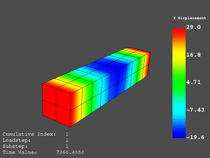
由于模型的几何图形包含在结果文件中，因此无需加载任何其他几何图形即可绘制结果。下面是使用 VTK 绘制的模态分析梁的一阶模态位移图。

在这里，我们绘制了一阶模态 （注意索引为 0） 在 x 方向上的位移：

result.plot_nodal_solution(0, 'x', label='Displacement')

通过设置相机和保存结果，可以非交互式绘制结果和保存屏幕截图。这有助于批处理结果的可视化和后期处理。

首先，从交互式绘图中获取摄像机的位置：

>>> cpos = result.plot_nodal_solution(0) # 感觉这个命令好像不对啊。 ——ff
>>> print(cpos)
[(5.2722879880979345, 4.308737919176047, 10.467694436036483),
 (0.5, 0.5, 2.5),
 (-0.2565529433509593, 0.9227952809887077, -0.28745339908049733)]

然后生成绘图：

result.plot_nodal_solution(0, 'x', label='Displacement', cpos=cpos,
                           screenshot='hexbeam_disp.png',
                           window_size=[800, 600], interactive=False)

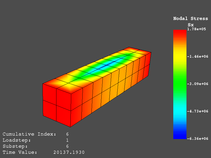
也可以使用下面的代码绘制应力图。节点应力的计算方法与 ANSYS 使用的方法相同，即通过求取所有附加单元在该节点处的应力平均值来确定每个节点处的应力。目前只能显示组件应力。

# 显示结果 6 的 X 方向节点平均应力
result.plot_nodal_stress(5, 'Sx')

节点应力也可通过以下非交互方式产生：

result.plot_nodal_stress(5, 'Sx', cpos=cpos, screenshot=beam_stress.png,
                         window_size=[800, 600], interactive=False)

动画模态

使用 `animate_nodal_solution 可将模态分析的模态振型制成动画：

result.animate_nodal_solution(0)

如果您希望将动画保存到文件中，请指定 movie_filename 参数并使用以下命令制作动画：

result.animate_nodal_solution(0, movie_filename='movie.mp4', cpos=cpos)

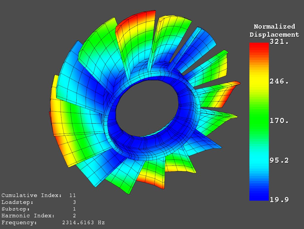
循环分析的结果

ansys-mapdl-reader 模块可以加载并显示循环分析的结果：

from ansys.mapdl import reader as pymapdl_reader

# load the result file
result = pymapdl_reader.read_binary('rotor.rst')

您可以通过打印结果头字典键 'ls_table' 和 'hindex' 来引用荷载阶跃表和谐波索引表：

>>> print(result.resultheader['ls_table'])
# load step, sub step, cumulative index
array([[ 1,  1,  1],
       [ 1,  2,  2],
       [ 1,  3,  3],
       [ 1,  4,  4],
       [ 1,  5,  5],
       [ 2,  1,  6],

>>> print(result.resultheader['hindex'])
array([0, 0, 0, 0, 0, 1, 1, 1, 1, 1, 2, 2, 2, 2, 2, 3, 3, 3, 3, 3, 4, 4, 4,
       4, 4, 5, 5, 5, 5, 5, 6, 6, 6, 6, 6, 7, 7, 7, 7, 7], dtype=int32)

其中每个谐波指数条目对应一个累积指数。例如，结果编号 11 是 2 次谐波指数的一阶模态：

>>> result.resultheader['ls_table'][10] # Result 11 (using zero based indexing)
array([ 3,  1, 11], dtype=int32)

>>> result.resultheader['hindex'][10]
2

另外，也可以使用以下方法获得结果编号：

>>> mode = 1
>>> harmonic_index = 2
>>> result.harmonic_index_to_cumulative(mode, harmonic_index)
24

使用这种索引方法，重复的模态由相同的模式索引进行索引。要访问另一个重复模态，请使用负谐波索引。如果结果不存在， ansys-mapdl-reader 将返回可用的模态：

>>> mode = 1
>>> harmonic_index = 20
>>> result.harmonic_index_to_cumulative(mode, harmonic_index)
Exception: Invalid mode for harmonic index 1
Available modes: [0 1 2 3 4 5 6 7 8 9]

循环分析的结果需要额外的后处理才能正确解释。模态振型作为模态解的实部和虚部的未处理部分存储在结果文件中。 ansys-mapdl-reader 将这些值合并为一个复数数组，然后返回该数组的实部结果。

>>> nnum, ms = result.nodal_solution(10) # mode shape of result 11
>>> print(ms[:3])
[[ 44.700, 45.953, 38.717]
 [ 42.339, 48.516, 52.475]
 [ 36.000, 33.121, 39.044]]

有时需要确定某一模态的最大位移。为此，可以用以下方法返回复数解：

nnum, ms = result.nodal_solution(0, as_complex=True)
norm = np.abs((ms*ms).sum(1)**0.5)
idx = np.nanargmax(norm)
ang = np.angle(ms[idx, 0])

# rotate the solution by the angle of the maximum nodal response
ms *= np.cos(ang) - 1j*np.sin(ang)

# get only the real response
ms = np.real(ms)

详情请参阅 help(result.nodal_solution) 。

扇形的 real displacement 始终是模态振型 ms 的实际分量，这可以通过将模态振型乘以给定相位的复数值来改变。

使用 plot_nodal_solution 也可以显示单个扇形的结果。

rnum = result.harmonic_index_to_cumulative(0, 2)
result.plot_nodal_solution(rnum, label='Displacement', expand=False)

可以通过修改 phase 选项来改变结果的相位。有关其实现的详情，请参阅 help(result.plot_nodal_solution) 。

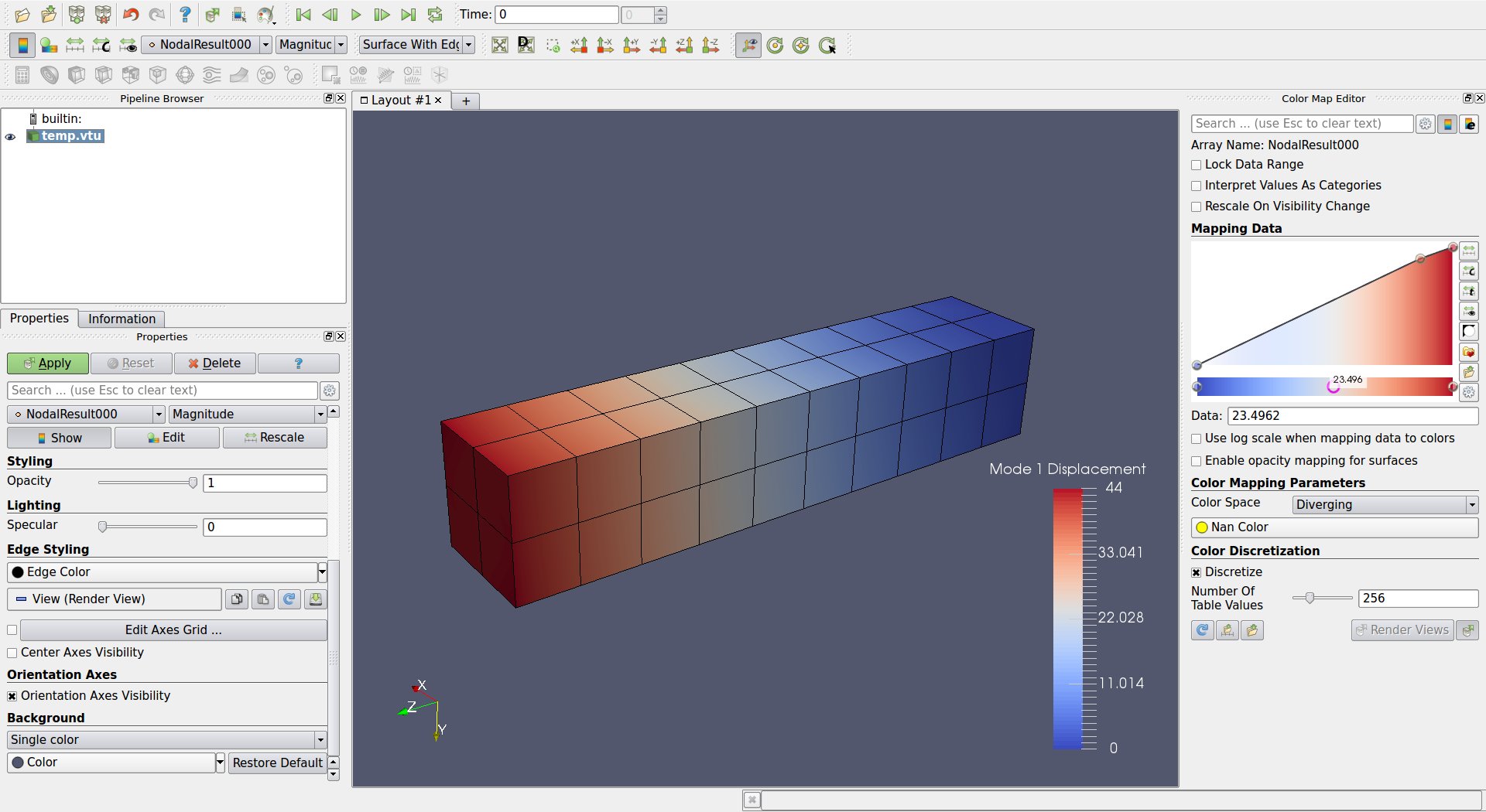
导出到 ParaView

ParaView 是一种可视化应用程序，可通过图形用户界面使用 VTK 快速生成绘图和图形。 ansys-mapdl-reader 可以将 MAPDL 结果文件转换为 ParaView 兼容文件，其中包含几何和节点分析结果：

from ansys.mapdl import reader as pymapdl_reader
from ansys.mapdl.reader import examples

# load example beam result file
result = pymapdl_reader.read_binary(examples.rstfile)

# save as a binary vtk xml file
result.save_as_vtk('beam.vtu') # 文件扩展名将选择要使用的写入器类型。``'.vtk'`` 将使用传统写入器，而``'.vtu'`` 将选择 VTK XML 写入器。

现在可以使用 ParaView 加载 vtk xml 文件了。该截图显示了在 ParaView 中绘制的结果文件中第一个结果的节点位移。 在 vtk 文件中，结果文件中的每个结果都有两个点数组（ NodalResult 和 nodal_stress ）。 节点结果值取决于分析类型，而节点应力始终是 Sx、Sy Sz、Sxy、Syz 和 Sxz 方向上的节点平均应力。

结果对象方法

class ansys.mapdl.reader.rst.Result(filename, read_mesh=True, parse_vtk=True, **kwargs)

Reads a binary ANSYS result file.

Parameters:

• filename (str, pathlib.Path, optional) – Filename of the ANSYS binary result file.

• ignore_cyclic (bool, optional) – Ignores any cyclic properties.

• read_mesh (bool, optional) – Debug parameter. Set to False to disable reading in the mesh from the result file.

• parse_vtk (bool, optional) – Set to False to skip the parsing the mesh as a VTK UnstructuredGrid, which might take a long time for large models.

Examples

>>> from ansys.mapdl import reader as pymapdl_reader
>>> rst = pymapdl_reader.read_binary('file.rst')

animate_nodal_displacement(rnum, comp='norm', node_components=None, element_components=None, sel_type_all=True, add_text=True, displacement_factor=0.1, n_frames=100, loop=True, movie_filename=None, progress_bar=True, **kwargs)

Animate nodal solution.

Assumes nodal solution is a displacement array from a modal or static solution.

rnumint or list

Cumulative result number with zero based indexing, or a list containing (step, substep) of the requested result.

compstr, default: “norm”

Scalar component to display. Options are 'x', 'y', 'z', and 'norm', and None.

node_componentslist, optional

Accepts either a string or a list strings of node components to plot. For example: ['MY_COMPONENT', 'MY_OTHER_COMPONENT]

element_componentslist, optional

Accepts either a string or a list strings of element components to plot. For example: ['MY_COMPONENT', 'MY_OTHER_COMPONENT]

sel_type_allbool, optional

If node_components is specified, plots those elements containing all nodes of the component. Default True.

add_textbool, optional

Adds information about the result.

displacement_factorfloat, optional

Increases or decreases displacement by a factor.

n_framesint, optional

Number of “frames” between each full cycle.

loopbool, optional

Loop the animation. Default True. Disable this to animate once and close. Automatically disabled when off_screen=True and movie_filename is set.

movie_filenamestr, pathlib.Path, optional

Filename of the movie to open. Filename should end in 'mp4', but other filetypes may be supported like "gif". See imagio.get_writer. A single loop of the mode will be recorded.

progress_barbool, default: True

Displays a progress bar when generating a movie while off_screen=True.

kwargsoptional keyword arguments

See pyvista.plot() for additional keyword arguments.

Examples

Animate the first result interactively.

>>> rst.animate_nodal_solution(0)

Animate second result while displaying the x scalars without looping

>>> rst.animate_nodal_solution(1, comp='x', loop=False)

Animate the second result and save as a movie.

>>> rst.animate_nodal_solution(0, movie_filename='disp.mp4')

Animate the second result and save as a movie in the background.

>>> rst.animate_nodal_solution(0, movie_filename='disp.mp4', off_screen=True)

Disable plotting within the notebook.

>>> rst.animate_nodal_solution(0, notebook=False)

animate_nodal_solution(rnum, comp='norm', node_components=None, element_components=None, sel_type_all=True, add_text=True, displacement_factor=0.1, n_frames=100, loop=True, movie_filename=None, progress_bar=True, **kwargs)

Animate nodal solution.

Assumes nodal solution is a displacement array from a modal or static solution.

rnumint or list

Cumulative result number with zero based indexing, or a list containing (step, substep) of the requested result.

compstr, default: “norm”

Scalar component to display. Options are 'x', 'y', 'z', and 'norm', and None.

node_componentslist, optional

Accepts either a string or a list strings of node components to plot. For example: ['MY_COMPONENT', 'MY_OTHER_COMPONENT]

element_componentslist, optional

Accepts either a string or a list strings of element components to plot. For example: ['MY_COMPONENT', 'MY_OTHER_COMPONENT]

sel_type_allbool, optional

If node_components is specified, plots those elements containing all nodes of the component. Default True.

add_textbool, optional

Adds information about the result.

displacement_factorfloat, optional

Increases or decreases displacement by a factor.

n_framesint, optional

Number of “frames” between each full cycle.

loopbool, optional

Loop the animation. Default True. Disable this to animate once and close. Automatically disabled when off_screen=True and movie_filename is set.

movie_filenamestr, pathlib.Path, optional

Filename of the movie to open. Filename should end in 'mp4', but other filetypes may be supported like "gif". See imagio.get_writer. A single loop of the mode will be recorded.

progress_barbool, default: True

Displays a progress bar when generating a movie while off_screen=True.

kwargsoptional keyword arguments

See pyvista.plot() for additional keyword arguments.

Examples

Animate the first result interactively.

>>> rst.animate_nodal_solution(0)

Animate second result while displaying the x scalars without looping

>>> rst.animate_nodal_solution(1, comp='x', loop=False)

Animate the second result and save as a movie.

>>> rst.animate_nodal_solution(0, movie_filename='disp.mp4')

Animate the second result and save as a movie in the background.

>>> rst.animate_nodal_solution(0, movie_filename='disp.mp4', off_screen=True)

Disable plotting within the notebook.

>>> rst.animate_nodal_solution(0, notebook=False)

animate_nodal_solution_set(rnums=None, comp='norm', node_components=None, element_components=None, sel_type_all=True, loop=True, movie_filename=None, add_text=True, fps=20, **kwargs)

Animate a set of nodal solutions.

Animates the scalars of all the result sets. Best when used with a series of static analyses.

rnumscollection.Iterable

Range or list containing the zero based indexed cumulative result numbers to animate.

compstr, optional

Scalar component to display. Options are 'x', 'y', 'z', and 'norm', and None. Not applicable for a thermal analysis.

node_componentslist, optional

Accepts either a string or a list strings of node components to plot. For example: ['MY_COMPONENT', 'MY_OTHER_COMPONENT]

element_componentslist, optional

Accepts either a string or a list strings of element components to plot. For example: ['MY_COMPONENT', 'MY_OTHER_COMPONENT]

sel_type_allbool, optional

If node_components is specified, plots those elements containing all nodes of the component. Default True.

loopbool, optional

Loop the animation. Default True. Disable this to animate once and close.

movie_filenamestr, optional

Filename of the movie to open. Filename should end in 'mp4', but other filetypes may be supported. See imagio.get_writer. A single loop of the mode will be recorded.

add_textbool, optional

Adds information about the result to the animation.

fpsint, optional

Frames per second. Defaults to 20 and limited to hardware capabilities and model density. Carries over to movies created by providing the movie_filename argument, but not to gifs.

kwargsoptional keyword arguments, optional

See help(pyvista.Plot) for additional keyword arguments.

Examples

Animate all results

>>> rst.animate_nodal_solution_set()

Animate every 50th result in a set of results and save to a gif. Use the “zx” camera position to view the ZX plane from the top down.

>>> rsets = range(0, rst.nsets, 50)
>>> rst.animate_nodal_solution_set(rsets,
...                                scalar_bar_args={'title': 'My Animation'},
...                                lighting=False, cpos='zx',
...                                movie_filename='example.gif')

property available_results

Available result types.

Examples

>>> rst.available_results
Available Results:
ENS : Nodal stresses
ENG : Element energies and volume
EEL : Nodal elastic strains
EPL : Nodal plastic strains
ETH : Nodal thermal strains (includes swelling strains)
EUL : Element euler angles
ENL : Nodal nonlinear items, e.g. equivalent plastic strains
EPT : Nodal temperatures
NSL : Nodal displacements
RF  : Nodal reaction forces

cs_4x4(cs_cord, as_vtk_matrix=False)

Return a 4x4 transformation matrix for a given coordinate system.

Parameters:

• cs_cord (int) – Coordinate system index.

• as_vtk_matrix (bool, default: False) – Return the transformation matrix as a vtkMatrix4x4.

Returns:

Matrix or vtkMatrix4x4 depending on the value of as_vtk_matrix.

Return type:

np.ndarray | vtk.vtkMatrix4x4

Notes

Values 11 and greater correspond to local coordinate systems

Examples

Return the transformation matrix for coordinate system 1.

>>> tmat = rst.cs_4x4(1)
>>> tmat
array([[1., 0., 0., 0.],
       [0., 1., 0., 0.],
       [0., 0., 1., 0.],
       [0., 0., 0., 1.]])

Return the transformation matrix for coordinate system 5. This corresponds to CSYS, 5, the cylindrical with global Cartesian Y as the axis of rotation.

>>> tmat = rst.cs_4x4(5)
>>> tmat
array([[ 1.,  0.,  0.,  0.],
       [ 0.,  0., -1.,  0.],
       [ 0.,  1.,  0.,  0.],
       [ 0.,  0.,  0.,  1.]])

cylindrical_nodal_stress(rnum, nodes=None)

Retrieves the stresses for each node in the solution in the cylindrical coordinate system as the following values:

R, THETA, Z, RTHETA, THETAZ, and RZ

The order of the results corresponds to the sorted node numbering.

Computes the nodal stress by averaging the stress for each element at each node. Due to the discontinuities across elements, stresses will vary based on the element they are evaluated from.

Parameters:

• rnum (int or list) – Cumulative result number with zero based indexing, or a list containing (step, substep) of the requested result.

• nodes (str, sequence of int or str, optional) –

  Select a limited subset of nodes. Can be a nodal component or array of node numbers. For example

  • "MY_COMPONENT"

  • ['MY_COMPONENT', 'MY_OTHER_COMPONENT]

  • np.arange(1000, 2001)

Returns:

• nnum (numpy.ndarray) – Node numbers of the result.

• stress (numpy.ndarray) – Stresses at R, THETA, Z, RTHETA, THETAZ, RZ averaged at each corner node where R is radial.

Examples

>>> from ansys.mapdl import reader as pymapdl_reader
>>> rst = pymapdl_reader.read_binary('file.rst')
>>> nnum, stress = rst.cylindrical_nodal_stress(0)

Return the cylindrical nodal stress just for the nodal component 'MY_COMPONENT'.

>>> nnum, stress = rst.cylindrical_nodal_stress(0, nodes='MY_COMPONENT')

Return the nodal stress just for the nodes from 20 through 50.

>>> nnum, stress = rst.cylindrical_nodal_stress(0, nodes=range(20, 51))

Notes

Nodes without a stress value will be NAN. Equivalent ANSYS commands: RSYS, 1 PRNSOL, S

property element_components

Dictionary of ansys element components from the result file.

Examples

>>> from ansys.mapdl import reader as pymapdl_reader
>>> from ansys.mapdl.reader import examples
>>> rst = pymapdl_reader.read_binary(examples.rstfile)
>>> rst.element_components
{'ECOMP1': array([17, 18, 21, 22, 23, 24, 25, 26, 27, 28, 29,
        30, 31, 32, 33, 34, 35, 36, 37, 38, 39, 40], dtype=int32),
'ECOMP2': array([ 1, 2, 3, 4, 5, 6, 7, 8, 9, 10, 11, 12, 13,
        14, 15, 16, 17, 18, 19, 20, 23, 24], dtype=int32),
'ELEM_COMP': array([ 5, 6, 7, 8, 9, 10, 11, 12, 13, 14, 15,
        16, 17, 18, 19, 20], dtype=int32)}

element_lookup(element_id)

Index of the element the element within the result mesh

element_solution_data(rnum, datatype, sort=True, **kwargs)

Retrieves element solution data. Similar to ETABLE.

Parameters:

• rnum (int or list) – Cumulative result number with zero based indexing, or a list containing (step, substep) of the requested result.

• datatype (str) –

  Element data type to retrieve.

  • EMS: misc. data

  • ENF: nodal forces

  • ENS: nodal stresses

  • ENG: volume and energies

  • EGR: nodal gradients

  • EEL: elastic strains

  • EPL: plastic strains

  • ECR: creep strains

  • ETH: thermal strains

  • EUL: euler angles

  • EFX: nodal fluxes

  • ELF: local forces

  • EMN: misc. non-sum values

  • ECD: element current densities

  • ENL: nodal nonlinear data

  • EHC: calculated heat generations

  • EPT: element temperatures

  • ESF: element surface stresses

  • EDI: diffusion strains

  • ETB: ETABLE items

  • ECT: contact data

  • EXY: integration point locations

  • EBA: back stresses

  • ESV: state variables

  • MNL: material nonlinear record

• sort (bool) – Sort results by element number. Default True.

• **kwargs (optional keyword arguments) – Hidden options for distributed result files.

Returns:

• enum (np.ndarray) – Element numbers.

• element_data (list) – List with one data item for each element.

• enode (list) – Node numbers corresponding to each element. results. One list entry for each element.

Notes

See ANSYS element documentation for available items for each element type. See:

https://www.mm.bme.hu/~gyebro/files/ans_help_v182/ans_elem/

Examples

Retrieve “LS” solution results from an PIPE59 element for result set 1

>>> enum, edata, enode = result.element_solution_data(0, datatype='ENS')
>>> enum[0]  # first element number
>>> enode[0]  # nodes belonging to element 1
>>> edata[0]  # data belonging to element 1
array([ -4266.19   ,   -376.18857,  -8161.785  , -64706.766  ,
        -4266.19   ,   -376.18857,  -8161.785  , -45754.594  ,
        -4266.19   ,   -376.18857,  -8161.785  ,      0.     ,
        -4266.19   ,   -376.18857,  -8161.785  ,  45754.594  ,
        -4266.19   ,   -376.18857,  -8161.785  ,  64706.766  ,
        -4266.19   ,   -376.18857,  -8161.785  ,  45754.594  ,
        -4266.19   ,   -376.18857,  -8161.785  ,      0.     ,
        -4266.19   ,   -376.18857,  -8161.785  , -45754.594  ,
        -4274.038  ,   -376.62527,  -8171.2603 ,   2202.7085 ,
       -29566.24   ,   -376.62527,  -8171.2603 ,   1557.55   ,
       -40042.613  ,   -376.62527,  -8171.2603 ,      0.     ,
       -29566.24   ,   -376.62527,  -8171.2603 ,  -1557.55   ,
        -4274.038  ,   -376.62527,  -8171.2603 ,  -2202.7085 ,
        21018.164  ,   -376.62527,  -8171.2603 ,  -1557.55   ,
        31494.537  ,   -376.62527,  -8171.2603 ,      0.     ,
        21018.164  ,   -376.62527,  -8171.2603 ,   1557.55   ],
      dtype=float32)

This data corresponds to the results you would obtain directly from MAPDL with ESOL commands:

>>> ansys.esol(nvar='2', elem=enum[0], node=enode[0][0], item='LS', comp=1)
>>> ansys.vget(par='SD_LOC1', ir='2', tstrt='1') # store in a variable
>>> ansys.read_float_parameter('SD_LOC1(1)')
-4266.19

element_stress(rnum, principal=False, in_element_coord_sys=False, **kwargs)

Retrieves the element component stresses.

Equivalent ANSYS command: PRESOL, S

Parameters:

• rnum (int or list) – Cumulative result number with zero based indexing, or a list containing (step, substep) of the requested result.

• principal (bool, optional) – Returns principal stresses instead of component stresses. Default False.

• in_element_coord_sys (bool, optional) – Returns the results in the element coordinate system. Default False and will return the results in the global coordinate system.

• **kwargs (optional keyword arguments) – Hidden options for distributed result files.

Returns:

• enum (np.ndarray) – ANSYS element numbers corresponding to each element.

• element_stress (list) – Stresses at each element for each node for Sx Sy Sz Sxy Syz Sxz or SIGMA1, SIGMA2, SIGMA3, SINT, SEQV when principal is True.

• enode (list) – Node numbers corresponding to each element’s stress results. One list entry for each element.

Examples

Element component stress for the first result set.

>>> rst.element_stress(0)

Element principal stress for the first result set.

>>> enum, element_stress, enode = result.element_stress(0, principal=True)

Notes

Shell stresses for element 181 are returned for top and bottom layers. Results are ordered such that the top layer and then the bottom layer is reported.

property filename: str

String form of the filename. This property is read-only.

property materials

Result file material properties.

Returns:

Dictionary of Materials. Keys are the material numbers, and each material is a dictionary of the material properrties of that material with only the valid entries filled.

Return type:

dict

Notes

Material properties:

• EX : Elastic modulus, element x direction (Force/Area)

• EY : Elastic modulus, element y direction (Force/Area)

• EZ : Elastic modulus, element z direction (Force/Area)

• ALPX : Coefficient of thermal expansion, element x direction (Strain/Temp)

• ALPY : Coefficient of thermal expansion, element y direction (Strain/Temp)

• ALPZ : Coefficient of thermal expansion, element z direction (Strain/Temp)

• REFT : Reference temperature (as a property) [TREF]

• PRXY : Major Poisson’s ratio, x-y plane

• PRYZ : Major Poisson’s ratio, y-z plane

• PRX Z : Major Poisson’s ratio, x-z plane

• NUXY : Minor Poisson’s ratio, x-y plane

• NUYZ : Minor Poisson’s ratio, y-z plane

• NUXZ : Minor Poisson’s ratio, x-z plane

• GXY : Shear modulus, x-y plane (Force/Area)

• GYZ : Shear modulus, y-z plane (Force/Area)

• GXZ : Shear modulus, x-z plane (Force/Area)

• DAMP : K matrix multiplier for damping [BETAD] (Time)

• MUCoefficient of friction (or, for FLUID29 and FLUID30

  elements, boundary admittance)

• DENS : Mass density (Mass/Vol)

• C : Specific heat (Heat/Mass*Temp)

• ENTH : Enthalpy (e DENS*C d(Temp)) (Heat/Vol)

• KXXThermal conductivity, element x direction

  (Heat*Length / (Time*Area*Temp))

• KYYThermal conductivity, element y direction

  (Heat*Length / (Time*Area*Temp))

• KZZThermal conductivity, element z direction

  (Heat*Length / (Time*Area*Temp))

• HF : Convection (or film) coefficient (Heat / (Time*Area*Temp))

• EMIS : Emissivity

• QRATE : Heat generation rate (MASS71 element only) (Heat/Time)

• VISC : Viscosity (Force*Time / Length2)

• SONC : Sonic velocity (FLUID29 and FLUID30 elements only) (Length/Time)

• RSVX : Electrical resistivity, element x direction (Resistance*Area / Length)

• RSVY : Electrical resistivity, element y direction (Resistance*Area / Length)

• RSVZ : Electrical resistivity, element z direction (Resistance*Area / Length)

• PERX : Electric permittivity, element x direction (Charge2 / (Force*Length))

• PERY : Electric permittivity, element y direction (Charge2 / (Force*Length))

• PERZ : Electric permittivity, element z direction (Charge2 / (Force*Length))

• MURX : Magnetic relative permeability, element x direction

• MURY : Magnetic relative permeability, element y direction

• MURZ : Magnetic relative permeability, element z direction

• MGXX : Magnetic coercive force, element x direction (Charge / (Length*Time))

• MGYY : Magnetic coercive force, element y direction (Charge / (Length*Time))

• MGZZ : Magnetic coercive force, element z direction (Charge / (Length*Time))

Materials may contain the key "stress_failure_criteria", which contains failure criteria information for temperature-dependent stress limits. This includes the following keys:

• XTEN : Allowable tensile stress or strain in the x-direction. (Must be positive.)

• XCMP : Allowable compressive stress or strain in the x-direction. (Defaults to negative of XTEN.)

• YTEN : Allowable tensile stress or strain in the y-direction. (Must be positive.)

• YCMP : Allowable compressive stress or strain in the y-direction. (Defaults to negative of YTEN.)

• ZTEN : Allowable tensile stress or strain in the z-direction. (Must be positive.)

• ZCMP : Allowable compressive stress or strain in the z-direction. (Defaults to negative of ZTEN.)

• XY : Allowable XY stress or shear strain. (Must be positive.)

• YZ : Allowable YZ stress or shear strain. (Must be positive.)

• XZ : Allowable XZ stress or shear strain. (Must be positive.)

• XYCP : XY coupling coefficient (Used only if Lab1 = S). Defaults to -1.0. [1]

• YZCP : YZ coupling coefficient (Used only if Lab1 = S). Defaults to -1.0. [1]

• XZCP : XZ coupling coefficient (Used only if Lab1 = S). Defaults to -1.0. [1]

• XZIT : XZ tensile inclination parameter for Puck failure index (default = 0.0)

• XZIC : XZ compressive inclination parameter for Puck failure index (default = 0.0)

• YZIT : YZ tensile inclination parameter for Puck failure index (default = 0.0)

• YZIC : YZ compressive inclination parameter for Puck failure index (default = 0.0)

Examples

Return the material properties from the example result file. Note that the keys of rst.materials is the material type.

>>> from ansys.mapdl import reader as pymapdl_reader
>>> from ansys.mapdl.reader import examples
>>> rst = pymapdl_reader.read_binary(examples.rstfile)
>>> rst.materials
{1: {'EX': 16900000.0, 'NUXY': 0.31, 'DENS': 0.00041408}}

property mesh

Mesh from result file.

Examples

>>> rst.mesh
ANSYS Mesh
  Number of Nodes:              1448
  Number of Elements:           226
  Number of Element Types:      1
  Number of Node Components:    0
  Number of Element Components: 0

property n_results

Number of results

property n_sector

Number of sectors

nodal_acceleration(rnum, in_nodal_coord_sys=False)

Nodal velocities for a given result set.

Parameters:

• rnum (int or list) – Cumulative result number with zero based indexing, or a list containing (step, substep) of the requested result.

• in_nodal_coord_sys (bool, optional) – When True, returns results in the nodal coordinate system. Default False.

Returns:

• nnum (int np.ndarray) – Node numbers associated with the results.

• result (float np.ndarray) – Array of nodal accelerations. Array is (nnod x sumdof), the number of nodes by the number of degrees of freedom which includes numdof and nfldof

Examples

>>> from ansys.mapdl import reader as pymapdl_reader
>>> rst = pymapdl_reader.read_binary('file.rst')
>>> nnum, data = rst.nodal_acceleration(0)

Notes

Some solution results may not include results for each node. These results are removed by and the node numbers of the solution results are reflected in nnum.

nodal_boundary_conditions(rnum)

Nodal boundary conditions for a given result number.

These nodal boundary conditions are generally set with the APDL command D. For example, D, 25, UX, 0.001

Parameters:

rnum (int or list) – Cumulative result number with zero based indexing, or a list containing (step, substep) of the requested result.

Returns:

• nnum (np.ndarray) – Node numbers of the nodes with boundary conditions.

• dof (np.ndarray) – Array of indices of the degrees of freedom of the nodes with boundary conditions. See rst.result_dof for the degrees of freedom associated with each index.

• bc (np.ndarray) – Boundary conditions.

Examples

Print the boundary conditions where: - Node 3 is fixed - Node 25 has UX=0.001 - Node 26 has UY=0.0011 - Node 27 has UZ=0.0012

>>> rst.nodal_boundary_conditions(0)
(array([ 3,  3,  3, 25, 26, 27], dtype=int32),
array([1, 2, 3, 1, 2, 3], dtype=int32),
array([0.    , 0.    , 0.    , 0.001 , 0.0011, 0.0012]))

nodal_displacement(rnum, in_nodal_coord_sys=False, nodes=None)

Returns the DOF solution for each node in the global cartesian coordinate system or nodal coordinate system.

Solution may be nodal temperatures or nodal displacements depending on the type of the solution.

Parameters:

• rnum (int or list) – Cumulative result number with zero based indexing, or a list containing (step, substep) of the requested result.

• in_nodal_coord_sys (bool, optional) – When True, returns results in the nodal coordinate system. Default False.

• nodes (str, sequence of int or str, optional) –

  Select a limited subset of nodes. Can be a nodal component or array of node numbers. For example

  • "MY_COMPONENT"

  • ['MY_COMPONENT', 'MY_OTHER_COMPONENT]

  • np.arange(1000, 2001)

Returns:

• nnum (int np.ndarray) – Node numbers associated with the results.

• result (float np.ndarray) – Array of nodal displacements or nodal temperatures. Array is (nnod x sumdof), the number of nodes by the number of degrees of freedom which includes numdof and nfldof

Examples

Return the nodal solution (in this case, displacement) for the first result of "file.rst".

>>> from ansys.mapdl import reader as pymapdl_reader
>>> rst = pymapdl_reader.read_binary('file.rst')
>>> nnum, data = rst.nodal_solution(0)

Return the nodal solution just for the nodal component 'MY_COMPONENT'.

>>> nnum, data = rst.nodal_solution(0, nodes='MY_COMPONENT')

Return the nodal solution just for the nodes from 20 through 50.

>>> nnum, data = rst.nodal_solution(0, nodes=range(20, 51))

Notes

Some solution results may not include results for each node. These results are removed by and the node numbers of the solution results are reflected in nnum.

nodal_elastic_strain(rnum, nodes=None)

Nodal component elastic strains. This record contains strains in the order X, Y, Z, XY, YZ, XZ, EQV.

Elastic strains can be can be nodal values extrapolated from the integration points or values at the integration points moved to the nodes.

Equivalent MAPDL command: PRNSOL, EPEL

Parameters:

• rnum (int or list) – Cumulative result number with zero based indexing, or a list containing (step, substep) of the requested result.

• nodes (str, sequence of int or str, optional) –

  Select a limited subset of nodes. Can be a nodal component or array of node numbers. For example

  • "MY_COMPONENT"

  • ['MY_COMPONENT', 'MY_OTHER_COMPONENT]

  • np.arange(1000, 2001)

Returns:

• nnum (np.ndarray) – MAPDL node numbers.

• elastic_strain (np.ndarray) – Nodal component elastic strains. Array is in the order X, Y, Z, XY, YZ, XZ, EQV.

Examples

Load the nodal elastic strain for the first result.

>>> from ansys.mapdl import reader as pymapdl_reader
>>> rst = pymapdl_reader.read_binary('file.rst')
>>> nnum, elastic_strain = rst.nodal_elastic_strain(0)

Return the nodal elastic strain just for the nodal component 'MY_COMPONENT'.

>>> nnum, elastic_strain = rst.nodal_elastic_strain(0, nodes='MY_COMPONENT')

Return the nodal elastic strain just for the nodes from 20 through 50.

>>> nnum, elastic_strain = rst.nodal_elastic_strain(0, nodes=range(20, 51))

Notes

Nodes without a strain will be NAN.

nodal_input_force(rnum)

Nodal input force for a given result number.

Nodal input force is generally set with the APDL command F. For example, F, 25, FX, 0.001

Parameters:

rnum (int or list) – Cumulative result number with zero based indexing, or a list containing (step, substep) of the requested result.

Returns:

• nnum (np.ndarray) – Node numbers of the nodes with nodal forces.

• dof (np.ndarray) – Array of indices of the degrees of freedom of the nodes with input force. See rst.result_dof for the degrees of freedom associated with each index.

• force (np.ndarray) – Nodal input force.

Examples

Print the nodal input force where: - Node 25 has FX=20 - Node 26 has FY=30 - Node 27 has FZ=40

>>> rst.nodal_input_force(0)
(array([ 71,  52, 127], dtype=int32),
 array([2, 1, 3], dtype=int32),
 array([30., 20., 40.]))

nodal_plastic_strain(rnum, nodes=None)

Nodal component plastic strains.

This record contains strains in the order: X, Y, Z, XY, YZ, XZ, EQV.

Plastic strains are always values at the integration points moved to the nodes.

Parameters:

• rnum (int or list) – Cumulative result number with zero based indexing, or a list containing (step, substep) of the requested result.

• nodes (str, sequence of int or str, optional) –

  Select a limited subset of nodes. Can be a nodal component or array of node numbers. For example

  • "MY_COMPONENT"

  • ['MY_COMPONENT', 'MY_OTHER_COMPONENT]

  • np.arange(1000, 2001)

Returns:

• nnum (np.ndarray) – MAPDL node numbers.

• plastic_strain (np.ndarray) – Nodal component plastic strains. Array is in the order X, Y, Z, XY, YZ, XZ, EQV.

Examples

Load the nodal plastic strain for the first solution.

>>> from ansys.mapdl import reader as pymapdl_reader
>>> rst = pymapdl_reader.read_binary('file.rst')
>>> nnum, plastic_strain = rst.nodal_plastic_strain(0)

Return the nodal plastic strain just for the nodal component 'MY_COMPONENT'.

>>> nnum, plastic_strain = rst.nodal_plastic_strain(0, nodes='MY_COMPONENT')

Return the nodal plastic strain just for the nodes from 20 through 50.

>>> nnum, plastic_strain = rst.nodal_plastic_strain(0, nodes=range(20, 51))

nodal_reaction_forces(rnum)

Nodal reaction forces.

Parameters:

rnum (int or list) – Cumulative result number with zero based indexing, or a list containing (step, substep) of the requested result.

Returns:

• rforces (np.ndarray) – Nodal reaction forces for each degree of freedom.

• nnum (np.ndarray) – Node numbers corresponding to the reaction forces. Node numbers may be repeated if there is more than one degree of freedom for each node.

• dof (np.ndarray) – Degree of freedom corresponding to each node using the MAPDL degree of freedom reference table. See rst.result_dof for the corresponding degrees of freedom for a given solution.

Examples

Get the nodal reaction forces for the first result and print the reaction forces of a single node.

>>> from ansys.mapdl import reader as pymapdl_reader
>>> rst = pymapdl_reader.read_binary('file.rst')
>>> rforces, nnum, dof = rst.nodal_reaction_forces(0)
>>> dof_ref = rst.result_dof(0)
>>> rforces[:3], nnum[:3], dof[:3], dof_ref
(array([  24102.21376091, -109357.01854005,   22899.5303263 ]),
 array([4142, 4142, 4142]),
 array([1, 2, 3], dtype=int32),
 ['UX', 'UY', 'UZ'])

nodal_solution(rnum, in_nodal_coord_sys=False, nodes=None)

Returns the DOF solution for each node in the global cartesian coordinate system or nodal coordinate system.

Solution may be nodal temperatures or nodal displacements depending on the type of the solution.

Parameters:

• rnum (int or list) – Cumulative result number with zero based indexing, or a list containing (step, substep) of the requested result.

• in_nodal_coord_sys (bool, optional) – When True, returns results in the nodal coordinate system. Default False.

• nodes (str, sequence of int or str, optional) –

  Select a limited subset of nodes. Can be a nodal component or array of node numbers. For example

  • "MY_COMPONENT"

  • ['MY_COMPONENT', 'MY_OTHER_COMPONENT]

  • np.arange(1000, 2001)

Returns:

• nnum (int np.ndarray) – Node numbers associated with the results.

• result (float np.ndarray) – Array of nodal displacements or nodal temperatures. Array is (nnod x sumdof), the number of nodes by the number of degrees of freedom which includes numdof and nfldof

Examples

Return the nodal solution (in this case, displacement) for the first result of "file.rst".

>>> from ansys.mapdl import reader as pymapdl_reader
>>> rst = pymapdl_reader.read_binary('file.rst')
>>> nnum, data = rst.nodal_solution(0)

Return the nodal solution just for the nodal component 'MY_COMPONENT'.

>>> nnum, data = rst.nodal_solution(0, nodes='MY_COMPONENT')

Return the nodal solution just for the nodes from 20 through 50.

>>> nnum, data = rst.nodal_solution(0, nodes=range(20, 51))

Notes

Some solution results may not include results for each node. These results are removed by and the node numbers of the solution results are reflected in nnum.

nodal_static_forces(rnum, nodes=None)

Return the nodal forces averaged at the nodes.

Nodal forces are computed on an element by element basis, and this method averages the nodal forces for each element for each node.

Parameters:

• rnum (int or list) – Cumulative result number with zero based indexing, or a list containing (step, substep) of the requested result.

• nodes (str, sequence of int or str, optional) –

  Select a limited subset of nodes. Can be a nodal component or array of node numbers. For example

  • "MY_COMPONENT"

  • ['MY_COMPONENT', 'MY_OTHER_COMPONENT]

  • np.arange(1000, 2001)

Returns:

• nnum (np.ndarray) – MAPDL node numbers.

• forces (np.ndarray) – Averaged nodal forces. Array is sized [nnod x numdof] where nnod is the number of nodes and numdof is the number of degrees of freedom for this solution.

Examples

Load the nodal static forces for the first result using the example hexahedral result file.

>>> from ansys.mapdl import reader as pymapdl_reader
>>> from ansys.mapdl.reader import examples
>>> rst = pymapdl_reader.read_binary(examples.rstfile)
>>> nnum, forces = rst.nodal_static_forces(0)

Return the nodal static forces just for the nodal component 'MY_COMPONENT'.

>>> nnum, forces = rst.nodal_static_forces(0, nodes='MY_COMPONENT')

Return the nodal static forces just for the nodes from 20 through 50.

>>> nnum, forces = rst.nodal_static_forces(0, nodes=range(20, 51))

Notes

Nodes without a a nodal will be NAN. These are generally midside (quadratic) nodes.

nodal_stress(rnum, nodes=None)

Retrieves the component stresses for each node in the solution.

The order of the results corresponds to the sorted node numbering.

Computes the nodal stress by averaging the stress for each element at each node. Due to the discontinuities across elements, stresses will vary based on the element they are evaluated from.

Parameters:

• rnum (int or list) – Cumulative result number with zero based indexing, or a list containing (step, substep) of the requested result.

• nodes (str, sequence of int or str, optional) –

  Select a limited subset of nodes. Can be a nodal component or array of node numbers. For example

  • "MY_COMPONENT"

  • ['MY_COMPONENT', 'MY_OTHER_COMPONENT]

  • np.arange(1000, 2001)

Returns:

• nnum (numpy.ndarray) – Node numbers of the result.

• stress (numpy.ndarray) – Stresses at X, Y, Z, XY, YZ, XZ averaged at each corner node.

Examples

>>> from ansys.mapdl import reader as pymapdl_reader
>>> rst = pymapdl_reader.read_binary('file.rst')
>>> nnum, stress = rst.nodal_stress(0)

Return the nodal stress just for the nodal component 'MY_COMPONENT'.

>>> nnum, stress = rst.nodal_stress(0, nodes='MY_COMPONENT')

Return the nodal stress just for the nodes from 20 through 50.

>>> nnum, stress = rst.nodal_solution(0, nodes=range(20, 51))

Notes

Nodes without a stress value will be NAN. Equivalent ANSYS command: PRNSOL, S

nodal_temperature(rnum, nodes=None, **kwargs)

Retrieves the temperature for each node in the solution.

The order of the results corresponds to the sorted node numbering.

Equivalent MAPDL command: PRNSOL, TEMP

Parameters:

• rnum (int or list) – Cumulative result number with zero based indexing, or a list containing (step, substep) of the requested result.

• nodes (str, sequence of int or str, optional) –

  Select a limited subset of nodes. Can be a nodal component or array of node numbers. For example

  • "MY_COMPONENT"

  • ['MY_COMPONENT', 'MY_OTHER_COMPONENT]

  • np.arange(1000, 2001)

Returns:

• nnum (numpy.ndarray) – Node numbers of the result.

• temperature (numpy.ndarray) – Temperature at each node.

Examples

>>> from ansys.mapdl import reader as pymapdl_reader
>>> rst = pymapdl_reader.read_binary('file.rst')
>>> nnum, temp = rst.nodal_temperature(0)

Return the temperature just for the nodal component 'MY_COMPONENT'.

>>> nnum, temp = rst.nodal_stress(0, nodes='MY_COMPONENT')

Return the temperature just for the nodes from 20 through 50.

>>> nnum, temp = rst.nodal_solution(0, nodes=range(20, 51))

nodal_thermal_strain(rnum, nodes=None)

Nodal component thermal strain.

This record contains strains in the order X, Y, Z, XY, YZ, XZ, EQV, and eswell (element swelling strain). Thermal strains are always values at the integration points moved to the nodes.

Equivalent MAPDL command: PRNSOL, EPTH, COMP

Parameters:

• rnum (int or list) – Cumulative result number with zero based indexing, or a list containing (step, substep) of the requested result.

• nodes (str, sequence of int or str, optional) –

  Select a limited subset of nodes. Can be a nodal component or array of node numbers. For example

  • "MY_COMPONENT"

  • ['MY_COMPONENT', 'MY_OTHER_COMPONENT]

  • np.arange(1000, 2001)

Returns:

• nnum (np.ndarray) – MAPDL node numbers.

• thermal_strain (np.ndarray) – Nodal component plastic strains. Array is in the order X, Y, Z, XY, YZ, XZ, EQV, ESWELL

Examples

Load the nodal thermal strain for the first solution.

>>> from ansys.mapdl import reader as pymapdl_reader
>>> rst = pymapdl_reader.read_binary('file.rst')
>>> nnum, thermal_strain = rst.nodal_thermal_strain(0)

Return the nodal thermal strain just for the nodal component 'MY_COMPONENT'.

>>> nnum, thermal_strain = rst.nodal_thermal_strain(0, nodes='MY_COMPONENT')

Return the nodal thermal strain just for the nodes from 20 through 50.

>>> nnum, thermal_strain = rst.nodal_thermal_strain(0, nodes=range(20, 51))

nodal_time_history(solution_type='NSL', in_nodal_coord_sys=False)

The DOF solution for each node for all result sets.

The nodal results are returned returned in the global cartesian coordinate system or nodal coordinate system.

Parameters:

• solution_type (str, optional) – The solution type. Must be either nodal displacements ('NSL'), nodal velocities ('VEL') or nodal accelerations ('ACC').

• in_nodal_coord_sys (bool, optional) – When True, returns results in the nodal coordinate system. Default False.

Returns:

• nnum (int np.ndarray) – Node numbers associated with the results.

• result (float np.ndarray) – Nodal solution for all result sets. Array is sized rst.nsets x nnod x Sumdof, which is the number of time steps by number of nodes by degrees of freedom.

nodal_velocity(rnum, in_nodal_coord_sys=False)

Nodal velocities for a given result set.

Parameters:

• rnum (int or list) – Cumulative result number with zero based indexing, or a list containing (step, substep) of the requested result.

• in_nodal_coord_sys (bool, optional) – When True, returns results in the nodal coordinate system. Default False.

Returns:

• nnum (int np.ndarray) – Node numbers associated with the results.

• result (float np.ndarray) – Array of nodal velocities. Array is (nnod x sumdof), the number of nodes by the number of degrees of freedom which includes numdof and nfldof

Examples

>>> from ansys.mapdl import reader as pymapdl_reader
>>> rst = pymapdl_reader.read_binary('file.rst')
>>> nnum, data = rst.nodal_velocity(0)

Notes

Some solution results may not include results for each node. These results are removed by and the node numbers of the solution results are reflected in nnum.

property node_components

Dictionary of ansys node components from the result file.

Examples

>>> from ansys.mapdl import reader as pymapdl_reader
>>> from ansys.mapdl.reader import examples
>>> rst = pymapdl_reader.read_binary(examples.rstfile)
>>> rst.node_components.keys()
dict_keys(['ECOMP1', 'ECOMP2', 'ELEM_COMP'])
>>> rst.node_components['NODE_COMP']
array([ 5, 6, 7, 8, 9, 10, 11, 12, 13, 14, 15, 16, 17, 18, 19,
      20], dtype=int32)

overwrite_element_solution_record(data, rnum, solution_type, element_id)

Overwrite element solution record.

This method replaces solution data for of an element at a result index for a given solution type. The number of items in data must match the number of items in the record.

If you are not sure how many records are in a given record, use element_solution_data to retrieve all the records for a given solution_type and check the number of items in the record.

Note: The record being replaced cannot be a compressed record. If the result file uses compression (default sparse compression as of 2019R1), you can disable this within MAPDL with: /FCOMP, RST, 0

Parameters:

• data (list or np.ndarray) – Data that will replace the existing records.

• rnum (int) – Zero based result number.

• solution_type (str) –

  Element data type to overwrite.

  • EMS: misc. data

  • ENF: nodal forces

  • ENS: nodal stresses

  • ENG: volume and energies

  • EGR: nodal gradients

  • EEL: elastic strains

  • EPL: plastic strains

  • ECR: creep strains

  • ETH: thermal strains

  • EUL: euler angles

  • EFX: nodal fluxes

  • ELF: local forces

  • EMN: misc. non-sum values

  • ECD: element current densities

  • ENL: nodal nonlinear data

  • EHC: calculated heat generations

  • EPT: element temperatures

  • ESF: element surface stresses

  • EDI: diffusion strains

  • ETB: ETABLE items

  • ECT: contact data

  • EXY: integration point locations

  • EBA: back stresses

  • ESV: state variables

  • MNL: material nonlinear record

• element_id (int) – Ansys element number (e.g. 1)

Examples

Overwrite the elastic strain record for element 1 for the first result with random data.

>>> from ansys.mapdl import reader as pymapdl_reader
>>> rst = pymapdl_reader.read_binary('file.rst')
>>> data = np.random.random(56)
>>> rst.overwrite_element_solution_data(data, 0, 'EEL', 1)

overwrite_element_solution_records(element_data, rnum, solution_type)

Overwrite element solution record.

This method replaces solution data for a set of elements at a result index for a given solution type. The number of items in data must match the number of items in the record.

If you are not sure how many records are in a given record, use element_solution_data to retrieve all the records for a given solution_type and check the number of items in the record.

Note: The record being replaced cannot be a compressed record. If the result file uses compression (default sparse compression as of 2019R1), you can disable this within MAPDL with: /FCOMP, RST, 0

Parameters:

• element_data (dict) – Dictionary of results that will replace the existing records.

• rnum (int) – Zero based result number.

• solution_type (str) –

  Element data type to overwrite.

  • EMS: misc. data

  • ENF: nodal forces

  • ENS: nodal stresses

  • ENG: volume and energies

  • EGR: nodal gradients

  • EEL: elastic strains

  • EPL: plastic strains

  • ECR: creep strains

  • ETH: thermal strains

  • EUL: euler angles

  • EFX: nodal fluxes

  • ELF: local forces

  • EMN: misc. non-sum values

  • ECD: element current densities

  • ENL: nodal nonlinear data

  • EHC: calculated heat generations

  • EPT: element temperatures

  • ESF: element surface stresses

  • EDI: diffusion strains

  • ETB: ETABLE items

  • ECT: contact data

  • EXY: integration point locations

  • EBA: back stresses

  • ESV: state variables

  • MNL: material nonlinear record

Examples

Overwrite the elastic strain record for elements 1 and 2 with for the first result with random data.

>>> from ansys.mapdl import reader as pymapdl_reader
>>> rst = pymapdl_reader.read_binary('file.rst')
>>> data = {1: np.random.random(56),
            2: np.random.random(56)}
>>> rst.overwrite_element_solution_data(data, 0, 'EEL')

parse_coordinate_system()

Reads in coordinate system information from a binary result file.

Returns:

c_systems – Dictionary containing one entry for each defined coordinate system. If no non-standard coordinate systems have been defined, an empty dictionary will be returned. First coordinate system is assumed to be global cartesian.

Return type:

dict

Notes

euler angles : [THXY, THYZ, THZX]

• First rotation about local Z (positive X toward Y).

• Second rotation about local X (positive Y toward Z).

• Third rotation about local Y (positive Z toward X).

PAR1 Used for elliptical, spheroidal, or toroidal systems. If KCS = 1 or 2, PAR1 is the ratio of the ellipse Y-axis radius to X-axis radius (defaults to 1.0 (circle)). If KCS = 3, PAR1 is the major radius of the torus.

PAR2 Used for spheroidal systems. If KCS = 2, PAR2 = ratio of ellipse Z-axis radius to X-axis radius (defaults to 1.0 (circle)).

Coordinate system type:

• 0: Cartesian

• 1: Cylindrical (circular or elliptical)

• 2: Spherical (or spheroidal)

• 3: Toroidal

parse_step_substep(user_input)

Converts (step, substep) to a cumulative index

property pathlib_filename: Path

Return the pathlib.Path version of the filename. This property can not be set.

plot(node_components=None, element_components=None, sel_type_all=True, **kwargs)

Plot result geometry

Parameters:

• node_components (list, optional) – Accepts either a string or a list strings of node components to plot. For example: ['MY_COMPONENT', 'MY_OTHER_COMPONENT]

• element_components (list, optional) – Accepts either a string or a list strings of element components to plot. For example: ['MY_COMPONENT', 'MY_OTHER_COMPONENT]

• sel_type_all (bool, optional) – If node_components is specified, plots those elements containing all nodes of the component. Default True.

• **kwargs (keyword arguments) – Optional keyword arguments. See help(pyvista.plot).

Returns:

cpos – List of camera position, focal point, and view up.

Return type:

list

Examples

>>> from ansys.mapdl import reader as pymapdl_reader
>>> rst = pymapdl_reader.read_binary('file.rst')
>>> rst.plot()

Plot just the element component ‘ROTOR_SHAFT’

>>> rst.plot(element_components='ROTOR_SHAFT')

Plot two node components >>> rst.plot(node_components=[‘MY_COMPONENT’, ‘MY_OTHER_COMPONENT’])

plot_cylindrical_nodal_stress(rnum, comp=None, show_displacement=False, displacement_factor=1, node_components=None, element_components=None, sel_type_all=True, treat_nan_as_zero=False, **kwargs)

Plot nodal_stress in the cylindrical coordinate system.

Parameters:

• rnum (int) – Result number

• comp (str, optional) – Stress component to display. Available options: - "R" - "THETA" - "Z" - "RTHETA" - "THETAZ" - "RZ"

• show_displacement (bool, optional) – Deforms mesh according to the result.

• displacement_factor (float, optional) – Increases or decreases displacement by a factor.

• node_components (list, optional) – Accepts either a string or a list strings of node components to plot. For example: ['MY_COMPONENT', 'MY_OTHER_COMPONENT]

• element_components (list, optional) – Accepts either a string or a list strings of element components to plot. For example: ['MY_COMPONENT', 'MY_OTHER_COMPONENT]

• sel_type_all (bool, optional) – If node_components is specified, plots those elements containing all nodes of the component. Default True.

• treat_nan_as_zero (bool, optional) – Treat NAN values (i.e. stresses at midside nodes) as zero when plotting.

• **kwargs (keyword arguments) – Optional keyword arguments. See help(pyvista.plot)

Examples

Plot nodal stress in the radial direction.

>>> from ansys.mapdl import reader as pymapdl_reader
>>> result = pymapdl_reader.read_binary('file.rst')
>>> result.plot_cylindrical_nodal_stress(0, 'R')

plot_element_result(rnum, result_type, item_index, in_element_coord_sys=False, **kwargs)

Plot an element result.

Parameters:

• rnum (int) – Result number.

• result_type (str) –

  Element data type to retrieve.

  • EMS: misc. data

  • ENF: nodal forces

  • ENS: nodal stresses

  • ENG: volume and energies

  • EGR: nodal gradients

  • EEL: elastic strains

  • EPL: plastic strains

  • ECR: creep strains

  • ETH: thermal strains

  • EUL: euler angles

  • EFX: nodal fluxes

  • ELF: local forces

  • EMN: misc. non-sum values

  • ECD: element current densities

  • ENL: nodal nonlinear data

  • EHC: calculated heat generations

  • EPT: element temperatures

  • ESF: element surface stresses

  • EDI: diffusion strains

  • ETB: ETABLE items

  • ECT: contact data

  • EXY: integration point locations

  • EBA: back stresses

  • ESV: state variables

  • MNL: material nonlinear record

• item_index (int) – Index of the data item for each node within the element.

• in_element_coord_sys (bool, optional) – Returns the results in the element coordinate system. Default False and will return the results in the global coordinate system.

Returns:

• nnum (np.ndarray) – ANSYS node numbers

• result (np.ndarray) – Array of result data

plot_nodal_displacement(rnum, comp=None, show_displacement=False, displacement_factor=1.0, node_components=None, element_components=None, sel_type_all=True, treat_nan_as_zero=False, **kwargs)

Plots the nodal solution.

Parameters:

• rnum (int or list) – Cumulative result number with zero based indexing, or a list containing (step, substep) of the requested result.

• comp (str, optional) – Display component to display. Options are 'X', 'Y', 'Z', 'NORM', or an available degree of freedom. Result may also include other degrees of freedom, check rst.result_dof for available degrees of freedoms for a given result. Defaults to "NORM" for a structural displacement result, and "TEMP" for a thermal result.

• show_displacement (bool, optional) – Deforms mesh according to the result.

• displacement_factor (float, optional) – Increases or decreases displacement by a factor.

• node_components (list, optional) – Accepts either a string or a list strings of node components to plot. For example: ['MY_COMPONENT', 'MY_OTHER_COMPONENT]

• element_components (list, optional) – Accepts either a string or a list strings of element components to plot. For example: ['MY_COMPONENT', 'MY_OTHER_COMPONENT]

• sel_type_all (bool, optional) – If node_components is specified, plots those elements containing all nodes of the component. Default True.

• treat_nan_as_zero (bool, optional) – Treat NAN values (i.e. stresses at midside nodes) as zero when plotting.

• **kwargs (keyword arguments) – Optional keyword arguments. See help(pyvista.plot).

Returns:

cpos – Camera position from vtk render window.

Return type:

list

Examples

Plot the nodal solution result 0 of verification manual example

>>> from ansys.mapdl import reader as pymapdl_reader
>>> from ansys.mapdl.reader import examples
>>> result = examples.download_verification_result(33)
>>> result.plot_nodal_solution(0)

Plot with a white background and showing edges

>>> result.plot_nodal_solution(0, background='w', show_edges=True)

plot_nodal_elastic_strain(rnum, comp, scalar_bar_args={'title': 'EQV Nodal Elastic Strain'}, show_displacement=False, displacement_factor=1, node_components=None, element_components=None, sel_type_all=True, treat_nan_as_zero=False, **kwargs)

Plot nodal elastic strain.

Parameters:

• rnum (int) – Result number

• comp (str, optional) – Elastic strain component to display. Available options: - "X" - "Y" - "Z" - "XY" - "YZ" - "XZ" - "EQV"

• show_displacement (bool, optional) – Deforms mesh according to the result.

• displacement_factor (float, optional) – Increases or decreases displacement by a factor.

• node_components (list, optional) – Accepts either a string or a list strings of node components to plot. For example: ['MY_COMPONENT', 'MY_OTHER_COMPONENT']

• element_components (list, optional) – Accepts either a string or a list strings of element components to plot. For example: ['MY_COMPONENT', 'MY_OTHER_COMPONENT']

• sel_type_all (bool, optional) – If node_components is specified, plots those elements containing all nodes of the component. Default True.

• treat_nan_as_zero (bool, optional) – Treat NAN values (i.e. stresses at midside nodes) as zero when plotting.

• **kwargs (keyword arguments) – Optional keyword arguments. See help(pyvista.plot)

Examples

Plot nodal elastic strain for a static pontoon model

>>> from ansys.mapdl import reader as pymapdl_reader
>>> from ansys.mapdl.reader import examples
>>> result = examples.download_pontoon()
>>> result.plot_nodal_elastic_strain(0)

plot_nodal_plastic_strain(rnum, comp, scalar_bar_args={'title': 'Nodal Plastic Strain'}, show_displacement=False, displacement_factor=1, node_components=None, element_components=None, sel_type_all=True, treat_nan_as_zero=False, **kwargs)

Plot nodal component plastic strain.

Parameters:

• rnum (int or list) – Cumulative result number with zero based indexing, or a list containing (step, substep) of the requested result.

• comp (str, optional) – Plastic strain component to display. Available options: - "X" - "Y" - "Z" - "XY" - "YZ" - "XZ" - "EQV"

• show_displacement (bool, optional) – Deforms mesh according to the result.

• displacement_factor (float, optional) – Increases or decreases displacement by a factor.

• node_components (list, optional) – Accepts either a string or a list strings of node components to plot. For example: ['MY_COMPONENT', 'MY_OTHER_COMPONENT]

• element_components (list, optional) – Accepts either a string or a list strings of element components to plot. For example: ['MY_COMPONENT', 'MY_OTHER_COMPONENT]

• sel_type_all (bool, optional) – If node_components is specified, plots those elements containing all nodes of the component. Default True.

• treat_nan_as_zero (bool, optional) – Treat NAN values (i.e. stresses at midside nodes) as zero when plotting.

• **kwargs (keyword arguments) – Optional keyword arguments. See help(pyvista.plot).

Examples

Plot plastic strain for a static pontoon model

>>> from ansys.mapdl import reader as pymapdl_reader
>>> from ansys.mapdl.reader import examples
>>> result = examples.download_pontoon()
>>> result.plot_nodal_plastic_strain(0)

plot_nodal_solution(rnum, comp=None, show_displacement=False, displacement_factor=1.0, node_components=None, element_components=None, sel_type_all=True, treat_nan_as_zero=False, **kwargs)

Plots the nodal solution.

Parameters:

• rnum (int or list) – Cumulative result number with zero based indexing, or a list containing (step, substep) of the requested result.

• comp (str, optional) – Display component to display. Options are 'X', 'Y', 'Z', 'NORM', or an available degree of freedom. Result may also include other degrees of freedom, check rst.result_dof for available degrees of freedoms for a given result. Defaults to "NORM" for a structural displacement result, and "TEMP" for a thermal result.

• show_displacement (bool, optional) – Deforms mesh according to the result.

• displacement_factor (float, optional) – Increases or decreases displacement by a factor.

• node_components (list, optional) – Accepts either a string or a list strings of node components to plot. For example: ['MY_COMPONENT', 'MY_OTHER_COMPONENT]

• element_components (list, optional) – Accepts either a string or a list strings of element components to plot. For example: ['MY_COMPONENT', 'MY_OTHER_COMPONENT]

• sel_type_all (bool, optional) – If node_components is specified, plots those elements containing all nodes of the component. Default True.

• treat_nan_as_zero (bool, optional) – Treat NAN values (i.e. stresses at midside nodes) as zero when plotting.

• **kwargs (keyword arguments) – Optional keyword arguments. See help(pyvista.plot).

Returns:

cpos – Camera position from vtk render window.

Return type:

list

Examples

Plot the nodal solution result 0 of verification manual example

>>> from ansys.mapdl import reader as pymapdl_reader
>>> from ansys.mapdl.reader import examples
>>> result = examples.download_verification_result(33)
>>> result.plot_nodal_solution(0)

Plot with a white background and showing edges

>>> result.plot_nodal_solution(0, background='w', show_edges=True)

plot_nodal_stress(rnum, comp=None, show_displacement=False, displacement_factor=1, node_components=None, element_components=None, sel_type_all=True, treat_nan_as_zero=False, **kwargs)

Plots the stresses at each node in the solution.

Parameters:

• rnum (int or list) – Cumulative result number with zero based indexing, or a list containing (step, substep) of the requested result.

• comp (str, optional) – Stress component to display. Available options: - "X" - "Y" - "Z" - "XY" - "YZ" - "XZ"

• node_components (list, optional) – Accepts either a string or a list strings of node components to plot. For example: ['MY_COMPONENT', 'MY_OTHER_COMPONENT]

• element_components (list, optional) – Accepts either a string or a list strings of element components to plot. For example: ['MY_COMPONENT', 'MY_OTHER_COMPONENT]

• sel_type_all (bool, optional) – If node_components is specified, plots those elements containing all nodes of the component. Default True.

• treat_nan_as_zero (bool, optional) – Treat NAN values (i.e. stresses at midside nodes) as zero when plotting.

• kwargs (keyword arguments) – Additional keyword arguments. See help(pyvista.plot)

Returns:

cpos – 3 x 3 vtk camera position.

Return type:

list

Examples

Plot the X component nodal stress while showing displacement.

>>> rst.plot_nodal_stress(0, comp='x', show_displacement=True)

plot_nodal_temperature(rnum, show_displacement=False, displacement_factor=1, node_components=None, element_components=None, sel_type_all=True, treat_nan_as_zero=False, **kwargs)

Plot nodal temperature

Parameters:

• rnum (int) – Result number

• show_displacement (bool, optional) – Deforms mesh according to the result.

• displacement_factor (float, optional) – Increases or decreases displacement by a factor.

• node_components (list, optional) – Accepts either a string or a list strings of node components to plot. For example: ['MY_COMPONENT', 'MY_OTHER_COMPONENT]

• element_components (list, optional) – Accepts either a string or a list strings of element components to plot. For example: ['MY_COMPONENT', 'MY_OTHER_COMPONENT]

• sel_type_all (bool, optional) – If node_components is specified, plots those elements containing all nodes of the component. Default True.

• treat_nan_as_zero (bool, optional) – Treat NAN values (i.e. stresses at midside nodes) as zero when plotting.

• **kwargs (keyword arguments) – Optional keyword arguments. See help(pyvista.plot)

Examples

Plot temperature of a result.

>>> from ansys.mapdl import reader as pymapdl_reader
>>> result = pymapdl_reader.read_binary('file.rst')
>>> result.plot_nodal_temperature(0)

Plot while showing edges and disabling lighting

>>> result.plot_nodal_temperature(0, show_edges=True, lighting=False)

plot_nodal_thermal_strain(rnum, comp=None, scalar_bar_args={'title': 'Nodal Thermal Strain'}, show_displacement=False, displacement_factor=1, node_components=None, element_components=None, sel_type_all=True, treat_nan_as_zero=False, **kwargs)

Plot nodal component thermal strains.

Equivalent MAPDL command: PLNSOL, EPTH, COMP

Parameters:

• rnum (int) – Result number

• comp (str, optional) – Thermal strain component to display. Available options: - "X" - "Y" - "Z" - "XY" - "YZ" - "XZ" - "EQV" - "ESWELL"

• show_displacement (bool, optional) – Deforms mesh according to the result.

• displacement_factor (float, optional) – Increases or decreases displacement by a factor.

• node_components (list, optional) – Accepts either a string or a list strings of node components to plot. For example: ['MY_COMPONENT', 'MY_OTHER_COMPONENT]

• element_components (list, optional) – Accepts either a string or a list strings of element components to plot. For example: ['MY_COMPONENT', 'MY_OTHER_COMPONENT]

• sel_type_all (bool, optional) – If node_components is specified, plots those elements containing all nodes of the component. Default True.

• treat_nan_as_zero (bool, optional) – Treat NAN values (i.e. stresses at midside nodes) as zero when plotting.

• **kwargs (keyword arguments) – Optional keyword arguments. See help(pyvista.plot)

Examples

Plot thermal strain for result 0 of verification manual example 33.

>>> from ansys.mapdl import reader as pymapdl_reader
>>> from ansys.mapdl.reader import examples
>>> result = examples.download_verification_result(33)
>>> result.plot_nodal_thermal_strain(0)

plot_principal_nodal_stress(rnum, comp=None, show_displacement=False, displacement_factor=1.0, node_components=None, element_components=None, sel_type_all=True, treat_nan_as_zero=False, **kwargs)

Plot the principal stress.

Parameters:

• rnum (int or list) – Cumulative result number with zero based indexing, or a list containing (step, substep) of the requested result.

• comp (string) –

  Stress component to plot. S1, S2, S3 principal stresses, SINT stress intensity, and SEQV equivalent stress.

  Stress type must be a string from the following list: ['S1', 'S2', 'S3', 'SINT', 'SEQV']

• show_displacement (bool, optional) – Deforms mesh according to the result.

• displacement_factor (float, optional) – Increases or decreases displacement by a factor.

• node_components (list, optional) – Accepts either a string or a list strings of node components to plot. For example: ['MY_COMPONENT', 'MY_OTHER_COMPONENT]

• element_components (list, optional) – Accepts either a string or a list strings of element components to plot. For example: ['MY_COMPONENT', 'MY_OTHER_COMPONENT]

• sel_type_all (bool, optional) – If node_components is specified, plots those elements containing all nodes of the component. Default True.

• treat_nan_as_zero (bool, optional) – Treat NAN values (i.e. stresses at midside nodes) as zero when plotting.

• kwargs (keyword arguments) – Additional keyword arguments. See help(pyvista.plot)

Returns:

cpos – VTK camera position.

Return type:

list

Examples

Plot the equivalent von mises stress.

>>> rst.plot_principal_nodal_stress(0, comp='SEQV')

principal_nodal_stress(rnum, nodes=None)

Computes the principal component stresses for each node in the solution.

Parameters:

rnum (int or list) – Cumulative result number with zero based indexing, or a list containing (step, substep) of the requested result.

Returns:

• nodenum (numpy.ndarray) – Node numbers of the result.

• pstress (numpy.ndarray) – Principal stresses, stress intensity, and equivalent stress. [sigma1, sigma2, sigma3, sint, seqv]

Examples

Load the principal nodal stress for the first solution.

>>> from ansys.mapdl import reader as pymapdl_reader
>>> rst = pymapdl_reader.read_binary('file.rst')
>>> nnum, stress = rst.principal_nodal_stress(0)

Notes

ANSYS equivalent of: PRNSOL, S, PRIN

which returns: S1, S2, S3 principal stresses, SINT stress intensity, and SEQV equivalent stress.

Internal averaging algorithm averages the component values from the elements at a common node and then calculates the principal using the averaged value.

See the MAPDL AVPRIN command for more details. ansys-mapdl-reader uses the default AVPRIN, 0 option.

result_dof(rnum)

Return a list of degrees of freedom for a given result number.

Parameters:

rnum (int or list) – Cumulative result number with zero based indexing, or a list containing (step, substep) of the requested result.

Returns:

dof – List of degrees of freedom.

Return type:

list

Examples

>>> rst.result_dof(0)
['UX', 'UY', 'UZ']

save_as_vtk(filename, rsets=None, result_types=['ENS'], progress_bar=True)

Writes results to a vtk readable file.

Nodal results will always be written.

The file extension will select the type of writer to use. '.vtk' will use the legacy writer, while '.vtu' will select the VTK XML writer.

Parameters:

• filename (str, pathlib.Path) – Filename of grid to be written. The file extension will select the type of writer to use. '.vtk' will use the legacy writer, while '.vtu' will select the VTK XML writer.

• rsets (collections.Iterable) – List of result sets to write. For example range(3) or [0].

• result_types (list) –

  Result type to write. For example ['ENF', 'ENS'] List of some or all of the following:

  • EMS: misc. data

  • ENF: nodal forces

  • ENS: nodal stresses

  • ENG: volume and energies

  • EGR: nodal gradients

  • EEL: elastic strains

  • EPL: plastic strains

  • ECR: creep strains

  • ETH: thermal strains

  • EUL: euler angles

  • EFX: nodal fluxes

  • ELF: local forces

  • EMN: misc. non-sum values

  • ECD: element current densities

  • ENL: nodal nonlinear data

  • EHC: calculated heat generations

  • EPT: element temperatures

  • ESF: element surface stresses

  • EDI: diffusion strains

  • ETB: ETABLE items

  • ECT: contact data

  • EXY: integration point locations

  • EBA: back stresses

  • ESV: state variables

  • MNL: material nonlinear record

• progress_bar (bool, optional) – Display a progress bar using tqdm.

Notes

Binary files write much faster than ASCII, but binary files written on one system may not be readable on other systems. Binary can only be selected for the legacy writer.

Examples

Write nodal results as a binary vtk file.

>>> rst.save_as_vtk('results.vtk')

Write using the xml writer

>>> rst.save_as_vtk('results.vtu')

Write only nodal and elastic strain for the first result

>>> rst.save_as_vtk('results.vtk', [0], ['EEL', 'EPL'])

Write only nodal results (i.e. displacements) for the first result.

>>> rst.save_as_vtk('results.vtk', [0], [])

property section_data

The section data from the result file

Returns:

section_data – Dictionary of the section data with the section numbers as keys.

Return type:

dict

Notes

There is limited documentation on how ANSYS stores the sections within a result file, and as such it may be difficult to interpret the section data for a given model.

solution_info(rnum)

Return an informative dictionary of solution data for a result.

Parameters:

rnum (int or list) – Cumulative result number with zero based indexing, or a list containing (step, substep) of the requested result.

Returns:

header – Double precision solution header data.

Return type:

dict

Examples

Extract the solution info from a sample example result file.

>>> from ansys.mapdl.reader import examples
>>> rst = examples.download_pontoon()
>>> rst.solution_info(0)
{'cgcent': [],
 'fatjack': [],
 'timfrq': 44.85185724963714,
 'lfacto': 1.0,
 'lfactn': 1.0,
 'cptime': 3586.4873046875,
 'tref': 71.6,
 'tunif': 71.6,
 'tbulk': 293.0,
 'volbase': 0.0,
 'tstep': 0.0,
 '__unused': 0.0,
 'accel_x': 0.0,
 'accel_y': 0.0,
 'accel_z': 0.0,
 'omega_v_x': 0.0,
 'omega_v_y': 0.0,
 'omega_v_z': 0.0,
 'omega_a_x': 0.0,
 'omega_a_y': 0.0,
 'omega_a_z': 0.0,
 'omegacg_v_x': 0.0,
 'omegacg_v_y': 0.0,
 'omegacg_v_z': 0.0,
 'omegacg_a_x': 0.0,
 'omegacg_a_y': 0.0,
 'omegacg_a_z': 0.0,
 'dval1': 0.0,
 'pCnvVal': 0.0}

Notes

The keys of the solution header are described below:

• timfrqTime value (or frequency value, for a modal or

  harmonic analysis)

• lfactothe “old” load factor (used in ramping a load

  between old and new values)

• lfactn : The “new” load factor

• cptime : Elapsed CPU time (in seconds)

• tref : The reference temperature

• tunif : The uniform temperature

• tbulk : Bulk temp for FLOTRAN film coefs.

• VolBase : Initial total volume for VOF

• tstep : Time Step size for FLOTRAN analysis

• 0.0 : Position not used

• accel : Linear acceleration terms

• omegaAngular velocity (first 3 terms) and angular acceleration

  (second 3 terms)

• omegacgAngular velocity (first 3 terms) and angular

  acceleration (second 3 terms) these velocity/acceleration terms are computed about the center of gravity

• cgcent : (X,y,z) location of center of gravity

• fatjack : Fatjack ocean wave data (wave height and period)

• dval1If pmeth=0: FATJACK ocean wave direction

  if pmeth=1: p-method convergence values

• pCnvVal : P-method convergence values

text_result_table(rnum)

Returns a text result table for plotting

property version

The version of MAPDL used to generate this result file.

Examples

>>> rst.version
20.1

write_tables(filename: str | Path)

Write binary tables to ASCII. Assumes int32

Parameters:

filename (str, pathlib.Path) – Filename to write the tables to.

Examples

>>> rst.write_tables('tables.txt')

class ansys.mapdl.reader.cyclic_reader.CyclicResult(filename)

Adds cyclic functionality to the result class

animate_nodal_displacement(rnum, comp='norm', displacement_factor=0.1, n_frames=180, add_text=True, loop=True, movie_filename=None, **kwargs)

Animate nodal solution. Assumes nodal solution is a displacement array from a modal solution.

rnumint or list

Cumulative result number with zero based indexing, or a list containing (step, substep) of the requested result.

compstr, optional

Component of displacement to display. Options are ‘x’, ‘y’, ‘z’, or ‘norm’, which correspond to the x , y, z, or the normalized direction (x**2 + y**2 + z**2)**0.5

displacement_factorfloat, optional

Increases or decreases displacement by a factor.

n_framesint, optional

Number of “frames” between each full cycle.

show_phasebool, optional

Shows the phase at each frame.

add_textbool, optional

Includes result information at the bottom left-hand corner of the plot.

interpolate_before_mapbool, optional

Leaving this at default generally results in a better plot.

movie_filenamestr, optional

Filename of the movie to open. Filename should end in mp4, but other filetypes may be supported. See imagio.get_writer. A single loop of the mode will be recorded.

kwargsoptional keyword arguments, optional

See help(pyvista.plot) for additional keyword arguments.

animate_nodal_solution(rnum, comp='norm', displacement_factor=0.1, n_frames=180, add_text=True, loop=True, movie_filename=None, **kwargs)

Animate nodal solution. Assumes nodal solution is a displacement array from a modal solution.

rnumint or list

Cumulative result number with zero based indexing, or a list containing (step, substep) of the requested result.

compstr, optional

Component of displacement to display. Options are ‘x’, ‘y’, ‘z’, or ‘norm’, which correspond to the x , y, z, or the normalized direction (x**2 + y**2 + z**2)**0.5

displacement_factorfloat, optional

Increases or decreases displacement by a factor.

n_framesint, optional

Number of “frames” between each full cycle.

show_phasebool, optional

Shows the phase at each frame.

add_textbool, optional

Includes result information at the bottom left-hand corner of the plot.

interpolate_before_mapbool, optional

Leaving this at default generally results in a better plot.

movie_filenamestr, optional

Filename of the movie to open. Filename should end in mp4, but other filetypes may be supported. See imagio.get_writer. A single loop of the mode will be recorded.

kwargsoptional keyword arguments, optional

See help(pyvista.plot) for additional keyword arguments.

property full_rotor

UnstructuredGrid of the full replicated rotor

harmonic_index_to_cumulative(hindex, mode)

Converts a harmonic index and a 0 index mode number to a cumulative result index.

Harmonic indices are stored as positive and negative pairs for modes other than 0 and N/nsectors.

Parameters:

• hindex (int) – Harmonic index. Must be less than or equal to nsectors/2. May be positive or negative

• mode (int) – Mode number. 0 based indexing. Access mode pairs by with a negative/positive harmonic index.

Returns:

rnum – Cumulative index number. Zero based indexing.

Return type:

int

property harmonic_indices

Harmonic indices of the result file.

Harmonic index is simply the Nodal Diameter of the mode. This is defined as the number of complete sine waves that pass through the circumference.

Examples

>>> rst.harmonic_indices
array([ 0,  0,  0,  0,  0,  0, -1,  1, -1,  1,  1, -1,
       -2,  2, -2,  2, -2,  2,  3,  3,  3,  3,  3,  3], dtype=int32)

property mode_table

Unique modes for cyclic results

nodal_displacement(rnum, phase=0, full_rotor=False, as_complex=False)

Return the DOF solution for each node in the global cartesian coordinate system.

Parameters:

• rnum (int or list) – Cumulative result number with zero based indexing, or a list containing (step, substep) of the requested result.

• phase (float, optional) – Phase to rotate sector result in radians.

• full_rotor (bool, optional) – Expands the single sector solution for the full rotor. Sectors are rotated counter-clockwise about the axis of rotation. Default False.

• as_complex (bool, optional) – Returns result as a complex number, otherwise as the real part rotated by phase. Default False.

Returns:

• nnum (numpy.ndarray) – Node numbers of master sector.

• result (numpy.ndarray) – Result is (nnod x numdof), nnod is the number of nodes in a sector and numdof is the number of degrees of freedom. When full_rotor is True the array will be (nSector x nnod x numdof).

Examples

Visualize the 1st nodal diameter mode.

>>> from ansys.mapdl import reader as pymapdl_reader
>>> from ansys.mapdl.reader import examples
>>> result = examples.download_academic_rotor()
>>> result.nodal_solution((2, 1))

Same result but uses Python (zero based) cumulative indexing

>>> result.nodal_solution(2)

Notes

Somewhere between v15.0 and v18.2 ANSYS stopped writing the duplicate sector to the result file and instead records results in pairs (i.e. harmonic index 1, -1).

nodal_elastic_strain(rnum, phase=0, as_complex=False, full_rotor=False)

Nodal component elastic strains. This record contains strains in the order X, Y, Z, XY, YZ, XZ, EQV.

Elastic strains can be can be nodal values extrapolated from the integration points or values at the integration points moved to the nodes.

Parameters:

• rnum (int or list) – Cumulative result number with zero based indexing, or a list containing (step, substep) of the requested result.

• phase (float) – Phase adjustment of the stress in radians.

• as_complex (bool, optional) – Reports stress as a complex result. Real and imaginary stresses correspond to the stress of the main and repeated sector. Stress can be “rotated” using the phase parameter.

• full_rotor (bool, optional) – Expands the results to the full rotor when True. Default False.

Returns:

• nodenum (numpy.ndarray) – Node numbers of the result.

• elastic_strain (numpy.ndarray) – Nodal component elastic strains. Array is in the order X, Y, Z, XY, YZ, XZ, EQV.

Examples

Load the nodal elastic strain for the first result.

>>> nnum, elastic_strain = rst.nodal_stress(0)

Notes

Nodes without a strain will be NAN.

nodal_plastic_strain(rnum, phase=0, as_complex=False, full_rotor=False)

Nodal component plastic strains. This record contains strains in the order X, Y, Z, XY, YZ, XZ, EQV.

Plastic strains can be can be nodal values extrapolated from the integration points or values at the integration points moved to the nodes.

Parameters:

• rnum (int or list) – Cumulative result number with zero based indexing, or a list containing (step, substep) of the requested result.

• phase (float) – Phase adjustment of the stress in degrees.

• as_complex (bool, optional) – Reports stress as a complex result. Real and imaginary stresses correspond to the stress of the main and repeated sector. Stress can be “rotated” using the phase parameter.

• full_rotor (bool, optional) – Expands the results to the full rotor when True. Default False.

Returns:

• nodenum (numpy.ndarray) – Node numbers of the result.

• plastic_strain (numpy.ndarray) – Nodal component plastic strains. Array is in the order X, Y, Z, XY, YZ, XZ, EQV.

Examples

Load the nodal plastic strain for the first result.

>>> nnum, plastic_strain = rst.nodal_stress(0)

Notes

Nodes without a strain will be NAN.

nodal_solution(rnum, phase=0, full_rotor=False, as_complex=False)

Return the DOF solution for each node in the global cartesian coordinate system.

Parameters:

• rnum (int or list) – Cumulative result number with zero based indexing, or a list containing (step, substep) of the requested result.

• phase (float, optional) – Phase to rotate sector result in radians.

• full_rotor (bool, optional) – Expands the single sector solution for the full rotor. Sectors are rotated counter-clockwise about the axis of rotation. Default False.

• as_complex (bool, optional) – Returns result as a complex number, otherwise as the real part rotated by phase. Default False.

Returns:

• nnum (numpy.ndarray) – Node numbers of master sector.

• result (numpy.ndarray) – Result is (nnod x numdof), nnod is the number of nodes in a sector and numdof is the number of degrees of freedom. When full_rotor is True the array will be (nSector x nnod x numdof).

Examples

Visualize the 1st nodal diameter mode.

>>> from ansys.mapdl import reader as pymapdl_reader
>>> from ansys.mapdl.reader import examples
>>> result = examples.download_academic_rotor()
>>> result.nodal_solution((2, 1))

Same result but uses Python (zero based) cumulative indexing

>>> result.nodal_solution(2)

Notes

Somewhere between v15.0 and v18.2 ANSYS stopped writing the duplicate sector to the result file and instead records results in pairs (i.e. harmonic index 1, -1).

nodal_stress(rnum, phase=0, as_complex=False, full_rotor=False)

Retrieves the component stresses for each node in the solution.

The order of the results corresponds to the sorted node numbering.

Computes the nodal stress by averaging the stress for each element at each node. Due to the discontinuities across elements, stresses will vary based on the element they are evaluated from.

Parameters:

• rnum (int or list) – Cumulative result number with zero based indexing, or a list containing (step, substep) of the requested result.

• phase (float) – Phase adjustment of the stress in degrees.

• as_complex (bool, optional) – Reports stress as a complex result. Real and imaginary stresses correspond to the stress of the main and repeated sector. Stress can be “rotated” using the phase parameter.

• full_rotor (bool, optional) – Expands the results to the full rotor when True. Default False.

Returns:

• nodenum (numpy.ndarray) – Node numbers of the result.

• stress (numpy.ndarray) – Stresses at Sx Sy Sz Sxy Syz Sxz averaged at each corner node. For the corresponding node numbers, see where result is the result object.

Examples

>>> nnum, stress = rst.nodal_stress(0)

Notes

Nodes without a stress value will be NAN.

nodal_temperature(rnum, full_rotor=False)

Retrieves the temperature for each node in the solution.

The order of the results corresponds to the sorted node numbering.

Equivalent MAPDL commands: PRNSOL, TEMP PRNSOL, BFE

Parameters:

• rnum (int or list) – Cumulative result number with zero based indexing, or a list containing (step, substep) of the requested result.

• full_rotor (bool, optional) – Expand sector solution to full rotor.

Returns:

• nnum (numpy.ndarray) – Node numbers of the result.

• temperature (numpy.ndarray) – Temperature at each node.

Examples

>>> nnum, stress = rst.nodal_temperature(0)

nodal_thermal_strain(rnum, phase=0, as_complex=False, full_rotor=False)

Nodal component thermal strains. This record contains strains in the order X, Y, Z, XY, YZ, XZ, EQV, and eswell (element swelling strain). Thermal strains are always values at the integration points moved to the nodes.

Parameters:

• rnum (int or list) – Cumulative result number with zero based indexing, or a list containing (step, substep) of the requested result.

• phase (float) – Phase adjustment of the stress in degrees.

• as_complex (bool, optional) – Reports stress as a complex result. Real and imaginary stresses correspond to the stress of the main and repeated sector. Stress can be “rotated” using the phase parameter.

• full_rotor (bool, optional) – Expands the results to the full rotor when True. Default False.

Returns:

• nodenum (numpy.ndarray) – Node numbers of the result.

• thermal_strain (np.ndarray) – Nodal component plastic strains. Array is in the order X, Y, Z, XY, YZ, XZ, EQV, ESWELL

Examples

Load the nodal thermal strain for the first result.

>>> nnum, thermal_strain = rst.nodal_thermal_strain(0)

Notes

Nodes without a strain will be NAN.

plot(**kwargs)

Plot the full rotor geometry.

Parameters:

kwargs (keyword arguments) – Additional keyword arguments. See help(pyvista.plot)

Returns:

cpos – List of camera position, focal point, and view up.

Return type:

list

Examples

>>> from ansys.mapdl.reader import examples
>>> rst = examples.download_academic_rotor()
>>> rst.plot()

Save a screenshot of the rotor

>>> rst.plot(screenshot='rotor.png')

plot_nodal_elastic_strain(rnum, comp=None, phase=0, full_rotor=True, show_displacement=False, displacement_factor=1, node_components=None, element_components=None, sel_type_all=True, add_text=True, overlay_wireframe=False, treat_nan_as_zero=False, **kwargs)

Plot nodal elastic strain.

Parameters:

• rnum (int or list) – Cumulative result number with zero based indexing, or a list containing (step, substep) of the requested result.

• comp (str, optional) – Elastic strain component to display. Available options: - "X" - "Y" - "Z" - "XY" - "YZ" - "XZ"

• phase (float, optional) – Phase angle of the modal result in radians. Only valid when full_rotor is True. Default 0

• full_rotor (bool, optional) – Expand the sector solution to the full rotor.

• show_displacement (bool, optional) – Deforms mesh according to the result.

• displacement_factor (float, optional) – Increases or decreases displacement by a factor.

• node_components (list, optional) – Accepts either a string or a list strings of node components to plot. For example: ['MY_COMPONENT', 'MY_OTHER_COMPONENT]

• element_components (list, optional) – Accepts either a string or a list strings of element components to plot. For example: ['MY_COMPONENT', 'MY_OTHER_COMPONENT]

• sel_type_all (bool, optional) – If node_components is specified, plots those elements containing all nodes of the component. Default True.

• treat_nan_as_zero (bool, optional) – Treat NAN values (i.e. stresses at midside nodes) as zero when plotting.

Returns:

cpos – Camera position from vtk render window.

Return type:

list

Examples

Plot nodal elastic strain for an academic rotor.

>>> result.plot_nodal_elastic_strain(0, 'X')

plot_nodal_plastic_strain(rnum, comp=None, phase=0, full_rotor=True, show_displacement=False, displacement_factor=1, node_components=None, element_components=None, sel_type_all=True, add_text=True, overlay_wireframe=False, treat_nan_as_zero=False, **kwargs)

Plot nodal plastic strain.

Parameters:

• rnum (int or list) – Cumulative result number with zero based indexing, or a list containing (step, substep) of the requested result.

• comp (str, optional) – Plastic strain component to display. Available options: - "X" - "Y" - "Z" - "XY" - "YZ" - "XZ"

• phase (float, optional) – Phase angle of the modal result in radians. Only valid when full_rotor is True. Default 0

• full_rotor (bool, optional) – Expand the sector solution to the full rotor.

• show_displacement (bool, optional) – Deforms mesh according to the result.

• displacement_factor (float, optional) – Increases or decreases displacement by a factor.

• node_components (list, optional) – Accepts either a string or a list strings of node components to plot. For example: ['MY_COMPONENT', 'MY_OTHER_COMPONENT]

• element_components (list, optional) – Accepts either a string or a list strings of element components to plot. For example: ['MY_COMPONENT', 'MY_OTHER_COMPONENT]

• sel_type_all (bool, optional) – If node_components is specified, plots those elements containing all nodes of the component. Default True.

• treat_nan_as_zero (bool, optional) – Treat NAN values (i.e. stresses at midside nodes) as zero when plotting.

Returns:

cpos – Camera position from vtk render window.

Return type:

list

Examples

Plot nodal plastic strain for an academic rotor

>>> result.plot_nodal_plastic_strain(0)

plot_nodal_solution(rnum, comp='norm', phase=0, full_rotor=True, show_displacement=False, displacement_factor=1.0, node_components=None, element_components=None, overlay_wireframe=False, add_text=True, sel_type_all=True, treat_nan_as_zero=False, **kwargs)

Plot the nodal solution (generally displacement).

Parameters:

• rnum (int or list) – Cumulative result number with zero based indexing, or a list containing (step, substep) of the requested result.

• comp (str, optional) – Display component to display. Options are ‘x’, ‘y’, ‘z’, and ‘norm’, corresponding to the x direction, y direction, z direction, and the normalized direction: (x**2 + y**2 + z**2)**0.5

• full_rotor (bool, optional) – Expand sector solution to full rotor.

• phase (float, optional) – Phase angle of the modal result in radians. Only valid when full_rotor is True. Default 0

• node_components (list, optional) – Accepts either a string or a list strings of node components to plot. For example: ['MY_COMPONENT', 'MY_OTHER_COMPONENT]

• element_components (list, optional) – Accepts either a string or a list strings of element components to plot. For example: ['MY_COMPONENT', 'MY_OTHER_COMPONENT]

• sel_type_all (bool, optional) – If node_components is specified, plots those elements containing all nodes of the component. Default True.

• treat_nan_as_zero (bool, optional) – Treat NAN values (i.e. stresses at midside nodes) as zero when plotting.

Returns:

cpos – Camera position from vtk render window.

Return type:

list

Examples

Plot the displacement of the first cyclic result.

>>> result.plot_nodal_solution(0)

plot_nodal_stress(rnum, comp=None, phase=0, full_rotor=True, show_displacement=False, displacement_factor=1, node_components=None, element_components=None, overlay_wireframe=False, add_text=True, sel_type_all=True, treat_nan_as_zero=False, **kwargs)

Plot nodal stress of a given component

Parameters:

• rnum (int or list) – Cumulative result number with zero based indexing, or a list containing (step, substep) of the requested result.

• comp (str, optional) – Stress component to display. Available options: - "X" - "Y" - "Z" - "XY" - "YZ" - "XZ"

• phase (float, optional) – Phase angle of the modal result in radians. Only valid when full_rotor is True. Default 0

• full_rotor (bool, optional) – Expand the sector solution to the full rotor.

• show_displacement (bool, optional) – Deforms mesh according to the result.

• displacement_factor (float, optional) – Increases or decreases displacement by a factor.

• node_components (list, optional) – Accepts either a string or a list strings of node components to plot. For example: ['MY_COMPONENT', 'MY_OTHER_COMPONENT]

• element_components (list, optional) – Accepts either a string or a list strings of element components to plot. For example: ['MY_COMPONENT', 'MY_OTHER_COMPONENT]

• sel_type_all (bool, optional) – If node_components is specified, plots those elements containing all nodes of the component. Default True.

• treat_nan_as_zero (bool, optional) – Treat NAN values (i.e. stresses at midside nodes) as zero when plotting.

Returns:

cpos – Camera position from vtk render window.

Return type:

list

Examples

Plot the "Z" nodal stress of the first cyclic result.

>>> result.plot_nodal_stress(0, comp="Z")

plot_nodal_temperature(rnum, phase=0, full_rotor=True, show_displacement=False, displacement_factor=1.0, node_components=None, overlay_wireframe=False, add_text=True, element_components=None, sel_type_all=True, treat_nan_as_zero=False, **kwargs)

Plot the nodal temperature.

Parameters:

• rnum (int or list) – Cumulative result number with zero based indexing, or a list containing (step, substep) of the requested result.

• full_rotor (bool, optional) – Expand the sector solution and plot the full rotor.

• phase (float, optional) – Phase angle of the modal result in radians. Only valid when full_rotor is True. Default 0

• node_components (list, optional) – Accepts either a string or a list strings of node components to plot. For example: ['MY_COMPONENT', 'MY_OTHER_COMPONENT]

• element_components (list, optional) – Accepts either a string or a list strings of element components to plot. For example: ['MY_COMPONENT', 'MY_OTHER_COMPONENT]

• sel_type_all (bool, optional) – If node_components is specified, plots those elements containing all nodes of the component. Default True.

• treat_nan_as_zero (bool, optional) – Treat NAN values (i.e. stresses at midside nodes) as zero when plotting.

Returns:

cpos – Camera position from vtk render window.

Return type:

list

Examples

Plot the nodal temperature of a rotor for the first result.

>>> result.plot_nodal_temperature(0)

plot_nodal_thermal_strain(rnum, comp=None, phase=0, full_rotor=True, show_displacement=False, displacement_factor=1, node_components=None, element_components=None, sel_type_all=True, add_text=True, overlay_wireframe=False, treat_nan_as_zero=False, **kwargs)

Plot nodal thermal strain.

Parameters:

• rnum (int or list) – Cumulative result number with zero based indexing, or a list containing (step, substep) of the requested result.

• comp (str, optional) – Thermal strain component to display. Available options: - "X" - "Y" - "Z" - "XY" - "YZ" - "XZ" - "EQV" - "ESWELL" (element swelling strain)

• phase (float, optional) – Phase angle of the modal result in radians. Only valid when full_rotor is True. Default 0.

• full_rotor (bool, optional) – Expand the sector solution to the full rotor.

• show_displacement (bool, optional) – Deforms mesh according to the result.

• displacement_factor (float, optional) – Increases or decreases displacement by a factor.

• node_components (list, optional) – Accepts either a string or a list strings of node components to plot. For example: ['MY_COMPONENT', 'MY_OTHER_COMPONENT]

• element_components (list, optional) – Accepts either a string or a list strings of element components to plot. For example: ['MY_COMPONENT', 'MY_OTHER_COMPONENT]

• sel_type_all (bool, optional) – If node_components is specified, plots those elements containing all nodes of the component. Default True.

• treat_nan_as_zero (bool, optional) – Treat NAN values (i.e. stresses at midside nodes) as zero when plotting.

Returns:

cpos – Camera position from vtk render window.

Return type:

list

Examples

Plot nodal thermal strain for an academic rotor

>>> rst.plot_nodal_thermal_strain(0)

plot_principal_nodal_stress(rnum, comp=None, phase=0, full_rotor=True, show_displacement=False, displacement_factor=1, node_components=None, element_components=None, sel_type_all=True, add_text=True, overlay_wireframe=False, treat_nan_as_zero=False, **kwargs)

Plot the nodal principal stress.

Parameters:

• rnum (int or list) – Cumulative result number with zero based indexing, or a list containing (step, substep) of the requested result.

• comp (string) –

  Stress component to plot. S1, S2, S3 principal stresses, SINT stress intensity, and SEQV equivalent stress.

  Stress type must be a string from the following list: ['S1', 'S2', 'S3', 'SINT', 'SEQV']

• phase (float, optional) – Phase angle of the modal result in radians. Only valid when full_rotor is True. Default 0

• full_rotor (bool, optional) – Expand sector solution to full rotor.

• show_displacement (bool, optional) – Deforms mesh according to the result.

• displacement_factor (float, optional) – Increases or decreases displacement by a factor.

• node_components (list, optional) – Accepts either a string or a list strings of node components to plot. For example: ['MY_COMPONENT', 'MY_OTHER_COMPONENT]

• sel_type_all (bool, optional) – If node_components is specified, plots those elements containing all nodes of the component. Default True.

• treat_nan_as_zero (bool, optional) – Treat NAN values (i.e. stresses at midside nodes) as zero when plotting.

• kwargs (keyword arguments) – Additional keyword arguments. See help(pyvista.plot)

Returns:

cpos – VTK camera position.

Return type:

list

Examples

Plot the von Mises stress of the first cyclic result.

>>> result.plot_principal_nodal_stress(0, comp='SEQV')

plot_sectors(**kwargs)

Plot the full rotor and individually color the sectors.

Parameters:

kwargs (keyword arguments) – Additional keyword arguments. See help(pyvista.plot)

Examples

>>> from ansys.mapdl.reader import examples
>>> rst = examples.download_academic_rotor()
>>> rst.plot_sectors()

Save a screenshot of the sectors

>>> rst.plot_sectors(screenshot='sectors.png')

principal_nodal_stress(rnum, phase=0, as_complex=False, full_rotor=False)

Computes the principal component stresses for each node in the solution.

Parameters:

• rnum (int or list) – Cumulative result number with zero based indexing, or a list containing (step, substep) of the requested result.

• phase (float) – Phase adjustment of the stress in degrees.

• as_complex (bool, optional) – Returns result as a complex number, otherwise as the real part rotated by phase. Default False.

• full_rotor (bool, optional) – Expand sector solution to full rotor.

Returns:

• nodenum (numpy.ndarray) – Node numbers of the result.

• pstress (numpy.ndarray) – Principal stresses, stress intensity, and equivalent stress. [sigma1, sigma2, sigma3, sint, seqv]

Notes

ANSYS equivalent of: PRNSOL, S, PRIN

which returns: S1, S2, S3 principal stresses, SINT stress intensity, and SEQV equivalent stress.