使用频率扫描 Krylov 方法进行谐波分析#
本例演示了如何使用 PyMAPDL 实现频率扫描克雷洛夫方法。有关更多信息,包括此方法背后的理论, 见 Frequency-Sweep Harmonic Analysis via the Krylov Method MAPDL 的 结构分析 指南中。
Overview#
本例使用频率扫描 Krylov (克雷洛夫)法对圆柱形声导管进行谐波分析,并研究系统在一定频率范围内的响应。
模型是一个圆柱形声导管,一端有压力负荷,另一端有输出阻抗。
这些是所需的主要步骤:
使用
KrylovSolver.gensubspace()方法生成 Krylov 子空间,用于谐波分析中的模型还原。使用
KrylovSolver.solve()方法缩小方程组,并在每个频率上求解。使用
KrylovSolver.expand()方法将缩小后的解扩展回 FE 空间。
Perform required imports#
Perform required imports and launch MAPDL.
import os
import numpy as np
import math
import matplotlib.pyplot as plt
from ansys.mapdl.core import launch_mapdl
from ansys.math.core.math import AnsMath

mapdl = launch_mapdl(nproc=4)
mapdl.clear()

# Importing and connecting PyAnsys Math with PyMAPDL
mm = AnsMath(mapdl)
Define parameters#
Define some geometry parameters and analysis settings. As mentioned earlier, the geometry
is a cylinder defined by its radius (cyl_r) and its length (cyl_L). The length
of the duct is such that three complete wavelengths (no_wl) can fit in its length
and can have ten elements per wavelength.
# Constants
pi = np.arccos(-1)
c0 = 340                         # speed of Sound (m/s)

# Materials
rho = 1.2                        # density
c0 = 340                         # speed of Sound
frq = 1000                       # excitation freq   Hz
visco = 0.9                      # viscosity

TP = 1/frq
WL = c0 * TP
no_wl = 3                        # no of wavelengths in space

cyl_L = no_wl * WL               # length of duct
cyl_r = 0.025 * cyl_L            # cross section of duct

nelem_wl = 10                    # no of elements per wavelength
tol_elem = nelem_wl * no_wl      # total number of elements across length
Define element type and materials#
Assign fluid medium (air) properties to the duct. This example
uses Fluid 220 (Keyopt(2)=1) with one degree of freedom per node (pressure),
with no FSI interface in the element.
mapdl.prep7()

mapdl.et(1,'FLUID220', kop2=1)   # uncoupled acoustic element without FSIs
mapdl.mp("DENS", 1, rho)
mapdl.mp("SONC", 1, c0)
mapdl.mp("VISC", 1, visco)
Define geometry#
Create a cylinder of the required dimensions and split it into four segments for uniform generation of the mesh in each segment.
# Set back to default
mapdl.csys(0)

# Rotate working plane for the cylinder generation
mapdl.wpcsys(-1)
mapdl.wprota(thzx=90)

# Generate a circular area with a specified radius
mapdl.cyl4(0, 0, cyl_r)

mapdl.wpcsys(-1)

# Extrude the circular area to generate a cylinder of specified length
mapdl.vext("ALL", dx=cyl_L)

# Split the cylinder into four segments to create a more uniform mesh
mapdl.vsbw("ALL", keep='DELETE')
mapdl.wprota(thzx=90)
mapdl.vsbw("ALL", keep='DELETE')

mapdl.wpcsys(-1)

# Create a component with the created volume
mapdl.cm('cm1', 'volu')
Create mesh#
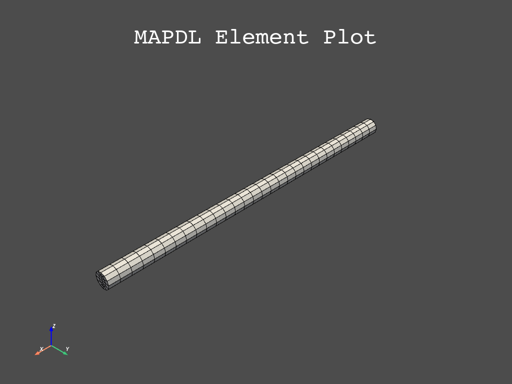
Create the mesh and plot the FE model.
# Select material and type
mapdl.mat(1)
mapdl.type(1)

# Select volume to mesh
mapdl.cmsel("S", "cm1")
To ensure that the volume is divided in tot_elem across its length, assign
a length element size constraint to the longitudinal lines.
# Select lines belonging to the volume
mapdl.aslv()
mapdl.lsla()

# Unselect lines at the top and bottom faces
mapdl.lsel("U", 'loc', 'x', 0)
mapdl.lsel("U", 'loc', 'x', cyl_L)

# Apply length constraint
mapdl.lesize('ALL',ndiv = tol_elem)
mapdl.lsla()

# Mesh
mapdl.vsweep('ALL')
mapdl.allsel()

# Plot the FE model
mapdl.eplot()

Define boundary conditions#
Apply pressure load on one end and output impedance on other end of the acoustic duct.
# Select areas to apply pressure to
mapdl.cmsel("S", "cm1")
mapdl.aslv()
mapdl.asel('R',"EXT")  # select external areas
mapdl.asel('R',"LOC","x",0)
mapdl.nsla('S',1)

# Apply pressure
mapdl.d('ALL','PRES', 1)

# Select nodes on the areas where impedance is to be applied
mapdl.cmsel("S", "cm1")
mapdl.aslv()
mapdl.asel('R',"EXT")
mapdl.asel('R',"LOC","x",cyl_L)
mapdl.nsla("S",1)

# Apply impedance
mapdl.sf("ALL","IMPD",1000)
mapdl.allsel()
Perform modal analysis#
Get the first 10 natural frequency modes of the acoustic duct.
# Modal Analysis
mapdl.slashsolu()
nev = 10 # Get the first 10 modes
output = mapdl.modal_analysis("DAMP", nmode=nev)
mapdl.finish()
mm.free()

k = mm.stiff(fname=f"{mapdl.jobname}.full")
M = mm.mass(fname=f"{mapdl.jobname}.full")
A = mm.mat(k.nrow, nev)
eigenvalues = mm.eigs(nev, k, M, phi=A, fmin=1.0)
The first ten modes are:
Mode number |
Frequency (Hz) |
|---|---|
1 |
83.33 |
2 |
250.00 |
3 |
416.67 |
4 |
583.34 |
5 |
750.03 |
6 |
916.74 |
7 |
1083.49 |
8 |
1250.32 |
9 |
1417.26 |
10 |
1584.36 |
Run harmonic analysis using Krylov method#
Perform the following steps to run the harmonic analysis using the frequency-sweep Krylov method.
Step 1: Generate FULL file and initialize the Krylov class object.
mapdl.run('/SOLU')
mapdl.antype('HARMIC')  # Set options for harmonic analysis
mapdl.hropt('KRYLOV')
mapdl.eqslv('SPARSE')
mapdl.harfrq(0,1000)    # Set beginning and ending frequency
mapdl.nsubst(100)       # Set the number of frequency increments
mapdl.wrfull(1)         # Generate FULL file and stop
mapdl.solve()
mapdl.finish()

dd = mapdl.krylov       # Initialize Krylov class object
Step 2: Generate a Krylov subspace of size/dimension 10 at frequency 500 Hz for model reduction.
Qz = dd.gensubspace(10, 500, check_orthogonality=True)
Obtain the shape of the generated subspace.
>>> print(Qz.shape)
(3240, 10)
Step 3: Reduce the system of equations and solve at each frequency from 0 Hz to 1000 Hz with ramped loading.
Yz = dd.solve(0, 1000, 100, ramped_load=True)
Obtain the shape of the reduced solution generated.
>>> print(Yz.shape)
(10, 100)
Step 4: Expand the reduced solution back to the FE space.
result = dd.expand(residual_computation=True, residual_algorithm="l2", return_solution = True)
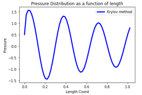
Plot the pressure distribution as a function of length#
Plot the pressure distribution over the length of the duct on nodes where Y, Z coordinates are zero.
# Select all nodes with Z and Y coordinate 0
mapdl.nsel("S", "LOC", "Z", 0)
mapdl.nsel("R", "LOC", "Y", 0)
mapdl.cm("node_comp", "NODES")
comp = mapdl.cmsel("S", "node_comp")
nodes = mapdl.db.nodes
ind, coords, angles = nodes.all_asarray()
Load the last result substep to get the pressure for each of the selected nodes.
x_data = []
y_data = []
substep_index = 99

def get_pressure_at(node, step=1):
    """Get pressure at a given node at a given step (by default first step)"""
    index_num = np.where(result[step]['node'] == node)
    return result[step][index_num]

for each_node, loc in zip(ind, coords):
    # Get pressure at the node
    pressure = get_pressure_at(each_node, substep_index)['x'][0]

    # Calculate amplitude at 60 deg
    magnitude = abs(pressure)
    phase = math.atan2(pressure.imag, pressure.real)
    pressure_a = magnitude * np.cos(np.deg2rad(60)+phase)

    # Store result for later plotting
    x_data.append(loc[0])  # X-Coordenate
    y_data.append(pressure_a)  # Nodal pressure at 60 degrees
Sort the results according to the X coordinate.
sorted_x_data, sorted_y_data = zip(*sorted(zip(x_data, y_data)))
Plot the calculated data.
plt.plot(sorted_x_data, sorted_y_data, linewidth= 3.0, color='b', label='Krylov method')

# Name the graph and the x-axis and y-axis
plt.title("Pressure distribution as a function of length")
plt.xlabel("Length coordinate")
plt.ylabel("Pressure")

# Add legend
plt.legend()

# Load the display window
plt.show()

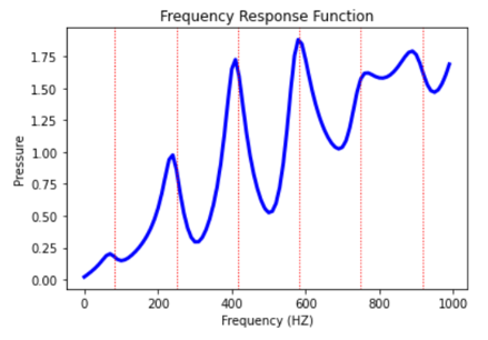
Plot the frequency response function#
Plot the frequency response function of any node along the length of the cylindrical duct. This code plots the frequency response function for a node along 0.2 in the X direction of the duct.
# Pick node closest to 0.2 in X direction, Y&Z = 0
node_number = mapdl.queries.node(0.2, 0, 0)
Get the response of the system for the selected node over a range of frequencies, such as 0 to 1000 Hz.
start_freq = 0
end_freq = 1000
num_steps = 100
step_val = (end_freq - start_freq) / num_steps
dic = {}

for freq in range(0, num_steps):
    pressure = get_pressure_at(node_number, freq)["x"]
    abs_pressure = abs(pressure)

    dic[start_freq] = abs_pressure
    start_freq += step_val
Sort the results.
frf_List = dic.items()
frf_List = sorted(frf_List)
frf_x, frf_y = zip(*frf_List)
Plot the frequency response function for the selected node.
plt.plot(frf_x, frf_y, linewidth=3.0, color="b")

# Plot the natural frequency as vertical lines on the FRF graph
for itr in range(0, 6):
    plt.axvline(
        x=eigenvalues[itr], ymin=0, ymax=2, color="r", linestyle="dotted", linewidth=1
    )

# Name the graph and the x-axis and y-axis
plt.title("Frequency Response Function")
plt.xlabel("Frequency (HZ)")
plt.ylabel("Pressure")

# Load the display window
plt.show()
